In this tutorial, you visualize geospatial analytics data from BigQuery by using a Colab notebook.
This tutorial uses the following BigQuery public datasets:
- San Francisco Ford GoBike Share
- San Francisco Neighborhoods
- San Francisco Police Department (SFPD) Reports
For information on accessing these public datasets, see Access public datasets in the Google Cloud console.
You use the public datasets to create the following visualizations:
- A scatter plot of all bike share stations from the Ford GoBike Share dataset
- Polygons in the San Francisco Neighborhoods dataset
- A choropleth map of the number of bike share stations by neighborhood
- A heatmap of incidents from the San Francisco Police Department Reports dataset
Objectives
- Set up authentication with Google Cloud and, optionally, Google Maps.
- Query data in BigQuery and download the results into Colab.
- Use Python data science tools to perform transformations and analyses.
- Create visualizations, including scatter plots, polygons, choropleths, and heatmaps.
Costs
In this document, you use the following billable components of Google Cloud:
To generate a cost estimate based on your projected usage,
use the pricing calculator.
When you finish the tasks that are described in this document, you can avoid continued billing by deleting the resources that you created. For more information, see Clean up.
Before you begin
- Sign in to your Google Cloud account. If you're new to Google Cloud, create an account to evaluate how our products perform in real-world scenarios. New customers also get $300 in free credits to run, test, and deploy workloads.
-
In the Google Cloud console, on the project selector page, select or create a Google Cloud project.
Roles required to select or create a project
- Select a project: Selecting a project doesn't require a specific IAM role—you can select any project that you've been granted a role on.
-
Create a project: To create a project, you need the Project Creator
(
roles/resourcemanager.projectCreator), which contains theresourcemanager.projects.createpermission. Learn how to grant roles.
-
Verify that billing is enabled for your Google Cloud project.
-
Enable the BigQuery and Google Maps JavaScript APIs.
Roles required to enable APIs
To enable APIs, you need the Service Usage Admin IAM role (
roles/serviceusage.serviceUsageAdmin), which contains theserviceusage.services.enablepermission. Learn how to grant roles. -
In the Google Cloud console, on the project selector page, select or create a Google Cloud project.
Roles required to select or create a project
- Select a project: Selecting a project doesn't require a specific IAM role—you can select any project that you've been granted a role on.
-
Create a project: To create a project, you need the Project Creator
(
roles/resourcemanager.projectCreator), which contains theresourcemanager.projects.createpermission. Learn how to grant roles.
-
Verify that billing is enabled for your Google Cloud project.
-
Enable the BigQuery and Google Maps JavaScript APIs.
Roles required to enable APIs
To enable APIs, you need the Service Usage Admin IAM role (
roles/serviceusage.serviceUsageAdmin), which contains theserviceusage.services.enablepermission. Learn how to grant roles. - Ensure that you have the necessary permissions to perform the tasks in this document.
Required roles
If you create a new project, you are the project owner, and you are granted all of the required IAM permissions that you need to complete this tutorial.
If you are using an existing project you need the following project-level role in order to run query jobs.
Make sure that you have the following role or roles on the project:
- BigQuery User (
roles/bigquery.user)
Check for the roles
-
In the Google Cloud console, go to the IAM page.
Go to IAM - Select the project.
-
In the Principal column, find all rows that identify you or a group that you're included in. To learn which groups you're included in, contact your administrator.
- For all rows that specify or include you, check the Role column to see whether the list of roles includes the required roles.
Grant the roles
-
In the Google Cloud console, go to the IAM page.
Go to IAM - Select the project.
- Click Grant access.
-
In the New principals field, enter your user identifier. This is typically the email address for a Google Account.
- In the Select a role list, select a role.
- To grant additional roles, click Add another role and add each additional role.
- Click Save.
For more information about roles in BigQuery, see Predefined IAM roles.
Create a Colab notebook
This tutorial builds a Colab notebook to visualize geospatial analytics data. You can open a prebuilt version of the notebook in Colab, Colab Enterprise, or BigQuery Studio by clicking the links at the top of the GitHub version of the tutorial— BigQuery Geospatial Visualization in Colab.
Open Colab.
In the Open notebook dialog, click New notebook.
Click
Untitled0.ipynband change the name of the notebook tobigquery-geo.ipynb.Select File > Save.
Authenticate with Google Cloud and Google Maps
This tutorial queries BigQuery datasets and uses the Google Maps JavaScript API. To use these resources, you authenticate the Colab runtime with Google Cloud and the Maps API.
Authenticate with Google Cloud
To insert a code cell, click Code.
To authenticate with your project, enter the following code:
# REQUIRED: Authenticate with your project.
GCP_PROJECT_ID = "PROJECT_ID"  #@param {type:"string"}

from google.colab import auth
from google.colab import userdata

auth.authenticate_user(project_id=GCP_PROJECT_ID)

# Set GMP_API_KEY to none
GMP_API_KEY = None
Replace PROJECT_ID with your project ID.
Click Run cell.
When prompted, click Allow to give Colab access to your credentials, if you agree.
On the Sign in with Google page, choose your account.
On the Sign in to Third-party authored notebook code page, click Continue.
On the Select what third-party authored notebook code can access, click Select all and then click Continue.
After you complete the authorization flow, no output is generated in your Colab notebook. The check mark beside the cell indicates that the code ran successfully.
Optional: Authenticate with Google Maps
If you use Google Maps Platform as the map provider for base maps, you must provide a Google Maps Platform API key. The notebook retrieves the key from your Colab Secrets.
This step is necessary only if you're using the Maps API. If you don't
authenticate with Google Maps Platform, pydeck uses the carto map instead.
Get your Google Maps API key by following the instructions on the Use API keys page in the Google Maps documentation.
Switch to your Colab notebook and then click Secrets.
Click Add new secret.
For Name, enter
GMP_API_KEY.For Value, enter the Maps API key value you generated previously.
Close the Secrets panel.
To insert a code cell, click Code.
To authenticate with the Maps API, enter the following code:
# Authenticate with the Google Maps JavaScript API.
GMP_API_SECRET_KEY_NAME = "GMP_API_KEY" #@param {type:"string"}

if GMP_API_SECRET_KEY_NAME:
  GMP_API_KEY = userdata.get(GMP_API_SECRET_KEY_NAME) if GMP_API_SECRET_KEY_NAME else None
else:
  GMP_API_KEY = None
When prompted, click Grant access to give the notebook access to your key, if you agree.
Click Run cell.
After you complete the authorization flow, no output is generated in your Colab notebook. The check mark beside the cell indicates that the code ran successfully.
Install Python packages and import data science libraries
In addition to the colabtools (google.colab)
Python modules, this tutorial uses several other Python packages and data
science libraries.
In this section, you install the pydeck and h3 packages. pydeck
provides high-scale spatial rendering in Python, powered by deck.gl.
h3-py provides Uber's H3 Hexagonal
Hierarchical Geospatial Indexing System in Python.
You then import the h3 and pydeck libraries and the following Python
geospatial libraries:
geopandasto extend the datatypes used bypandasto allow spatial operations on geometric types.shapelyfor manipulation and analysis of individual planar geometric objects.brancato generate HTML and JavaScript colormaps.geemap.deckfor visualization withpydeckandearthengine-api.
After importing the libraries, you enable interactive tables for pandas
DataFrames in Colab.
Install the pydeck and h3 packages
To insert a code cell, click Code.
To install the
pydeckandh3packages, enter the following code:# Install pydeck and h3. !pip install pydeck>=0.9 h3>=4.2
Click Run cell.
After you complete the installation, no output is generated in your Colab notebook. The check mark beside the cell indicates that the code ran successfully.
Import the Python libraries
To insert a code cell, click Code.
To import the Python libraries, enter the following code:
# Import data science libraries.
import branca
import geemap.deck as gmdk
import h3
import pydeck as pdk
import geopandas as gpd
import shapely
Click Run cell.
After you run the code, no output is generated in your Colab notebook. The check mark beside the cell indicates that the code ran successfully.
Enable interactive tables for pandas DataFrames
To insert a code cell, click Code.
To enable
pandasDataFrames, enter the following code:# Enable displaying pandas data frames as interactive tables by default. from google.colab import data_table data_table.enable_dataframe_formatter()
Click Run cell.
After you run the code, no output is generated in your Colab notebook. The check mark beside the cell indicates that the code ran successfully.
Create a shared routine
In this section, you create a shared routine that renders layers on a base map.
To insert a code cell, click Code.
To create a shared routine for rendering layers on a map, enter the following code:
# Set Google Maps as the base map provider.
MAP_PROVIDER_GOOGLE = pdk.bindings.base_map_provider.BaseMapProvider.GOOGLE_MAPS.value

# Shared routine for rendering layers on a map using geemap.deck.
def display_pydeck_map(layers, view_state, **kwargs):
  deck_kwargs = kwargs.copy()

  # Use Google Maps as the base map only if the API key is provided.
  if GMP_API_KEY:
    deck_kwargs.update({
      "map_provider": MAP_PROVIDER_GOOGLE,
      "map_style": pdk.bindings.map_styles.GOOGLE_ROAD,
      "api_keys": {MAP_PROVIDER_GOOGLE: GMP_API_KEY},
    })

  m = gmdk.Map(initial_view_state=view_state, ee_initialize=False, **deck_kwargs)

  for layer in layers:
    m.add_layer(layer)
  return m
Click Run cell.
After you run the code, no output is generated in your Colab notebook. The check mark beside the cell indicates that the code ran successfully.
Create a scatter plot
In this section, you create a scatter plot of all bike share stations in the
San Francisco Ford GoBike Share public dataset by retrieving data from the
bigquery-public-data.san_francisco_bikeshare.bikeshare_station_info table. The
scatter plot is created using a layer
and a scatterplot layer
from the deck.gl framework.
Scatter plots are useful when you need to review a subset of individual points (also known as spot checking).
The following example demonstrates how to use a layer and a scatterplot layer to render individual points as circles.
To insert a code cell, click Code.
To query the San Francisco Ford GoBike Share public dataset, enter the following code. This code uses the
%%bigquerymagic function to run the query and return the results in a DataFrame:# Query the station ID, station name, station short name, and station # geometry from the bike share dataset. # NOTE: In this tutorial, the denormalized 'lat' and 'lon' columns are # ignored. They are decomposed components of the geometry. %%bigquery gdf_sf_bikestations --project {GCP_PROJECT_ID} --use_geodataframe station_geom SELECT station_id, name, short_name, station_geom FROM `bigquery-public-data.san_francisco_bikeshare.bikeshare_station_info`
Click Run cell.
The output is similar to the following:
Job ID 12345-1234-5678-1234-123456789 successfully executed: 100%To insert a code cell, click Code.
To get a summary of the DataFrame, including columns and data types, enter the following code:
# Get a summary of the DataFrame
gdf_sf_bikestations.info()
Click Run cell.
The output should look like the following:
<class 'geopandas.geodataframe.GeoDataFrame'>
RangeIndex: 472 entries, 0 to 471
Data columns (total 4 columns):
#   Column        Non-Null Count  Dtype
---  ------        --------------  -----
0   station_id    472 non-null    object
1   name          472 non-null    object
2   short_name    472 non-null    object
3   station_geom  472 non-null    geometry
dtypes: geometry(1), object(3)
memory usage: 14.9+ KB
To insert a code cell, click Code.
To preview the first five rows of the DataFrame, enter the following code:
# Preview the first five rows
gdf_sf_bikestations.head()
Click Run cell.
The output is similar to the following:
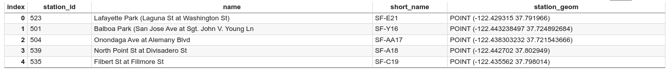
Rendering the points requires you to extract the longitude and latitude
as x and y coordinates from the station_geom column in the bike share dataset.
Since gdf_sf_bikestations is a geopandas.GeoDataFrame, coordinates are
accessed directly from its station_geom geometry column. You can retrieve
the longitude using the column's .x attribute and the latitude using its .y
attribute. Then, you can store them in new longitude and latitude columns.
To insert a code cell, click Code.
To extract the longitude and latitude values from the
station_geomcolumn, enter the following code:# Extract the longitude (x) and latitude (y) from station_geom. gdf_sf_bikestations["longitude"] = gdf_sf_bikestations["station_geom"].x gdf_sf_bikestations["latitude"] = gdf_sf_bikestations["station_geom"].y
Click Run cell.
After you run the code, no output is generated in your Colab notebook. The check mark beside the cell indicates that the code ran successfully.
To insert a code cell, click Code.
To render the scatter plot of bike share stations based on the longitude and latitude values you extracted previously, enter the following code:
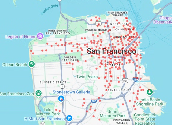
# Render a scatter plot using pydeck with the extracted longitude and
# latitude columns in the gdf_sf_bikestations geopandas.GeoDataFrame.
scatterplot_layer = pdk.Layer(
  "ScatterplotLayer",
  id="bike_stations_scatterplot",
  data=gdf_sf_bikestations,
  get_position=['longitude', 'latitude'],
  get_radius=100,
  get_fill_color=[255, 0, 0, 140],  # Adjust color as desired
  pickable=True,
)

view_state = pdk.ViewState(latitude=37.77613, longitude=-122.42284, zoom=12)
display_pydeck_map([scatterplot_layer], view_state)
Click Run cell.
The output is similar to the following:
Visualize polygons
Geospatial analytics lets you analyze and visualize geospatial data in
BigQuery by using GEOGRAPHY data types and GoogleSQL
geography functions.
The GEOGRAPHY data type
in geospatial analytics is a collection of points, linestrings, and
polygons, which is represented as a point set, or a subset of the surface of the
Earth. A GEOGRAPHY type can contain objects such as the following:
- Points
- Lines
- Polygons
- Multipolygons
For a list of all supported objects, see the GEOGRAPHY type
documentation.
If you are provided geospatial data without knowing the expected shapes, you can
visualize the data to discover the shapes. You can visualize shapes by
converting the geographic data to GeoJSON format. You
can then visualize the GeoJSON data using a GeoJSON layer
from the deck.gl framework.
In this section, you query geographic data in the San Francisco Neighborhoods dataset and then visualize the polygons.
To insert a code cell, click Code.
To query the geographic data from the
bigquery-public-data.san_francisco_neighborhoods.boundariestable in the San Francisco Neighborhoods dataset, enter the following code. This code uses the%%bigquerymagic function to run the query and return the results in a DataFrame:# Query the neighborhood name and geometry from the San Francisco # neighborhoods dataset. %%bigquery gdf_sanfrancisco_neighborhoods --project {GCP_PROJECT_ID} --use_geodataframe geometry SELECT neighborhood, neighborhood_geom AS geometry FROM `bigquery-public-data.san_francisco_neighborhoods.boundaries`
Click Run cell.
The output is similar to the following:
Job ID 12345-1234-5678-1234-123456789 successfully executed: 100%To insert a code cell, click Code.
To get a summary of the DataFrame, enter the following code:
# Get a summary of the DataFrame
gdf_sanfrancisco_neighborhoods.info()
Click Run cell.
The results should look like the following:
<class 'geopandas.geodataframe.GeoDataFrame'>
RangeIndex: 117 entries, 0 to 116
Data columns (total 2 columns):
#   Column        Non-Null Count  Dtype
---  ------        --------------  -----
0   neighborhood  117 non-null    object
1   geometry      117 non-null    geometry
dtypes: geometry(1), object(1)
memory usage: 2.0+ KB
To preview the first row of the DataFrame, enter the following code:
# Preview the first row
gdf_sanfrancisco_neighborhoods.head(1)
Click Run cell.
The output is similar to the following:
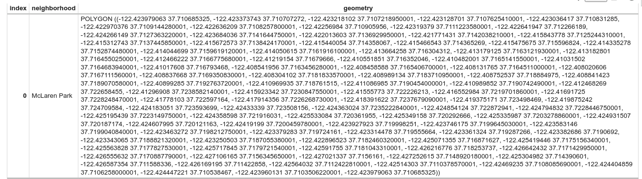
In the results, notice that the data is a polygon.
To insert a code cell, click Code.
To visualize the polygons, enter the following code.
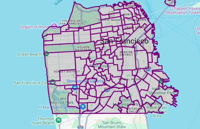
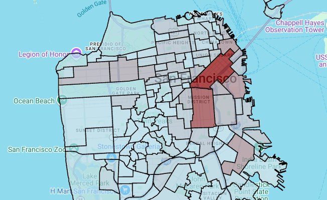
pydeckis used to convert eachshapelyobject instance in the geometry column intoGeoJSONformat:# Visualize the polygons. geojson_layer = pdk.Layer( 'GeoJsonLayer', id="sf_neighborhoods", data=gdf_sanfrancisco_neighborhoods, get_line_color=[127, 0, 127, 255], get_fill_color=[60, 60, 60, 50], get_line_width=100, pickable=True, stroked=True, filled=True, ) view_state = pdk.ViewState(latitude=37.77613, longitude=-122.42284, zoom=12) display_pydeck_map([geojson_layer], view_state)
Click Run cell.
The output is similar to the following:
Create a choropleth map
If you are exploring data with polgyons that are difficult to convert to
GeoJSON format, you can use a polygon layer
from the deck.gl framework instead. A polygon layer can process input data of
specific types such as an array of points.
In this section, you use a polygon layer to render an array of points and use the results to render a choropleth map. The choropleth map shows the density of bike share stations by neighborhood by joining data from the San Francisco Neighborhoods dataset with the San Francisco Ford GoBike Share dataset.
To insert a code cell, click Code.
To aggregate and count the number of stations per neighborhood and to create a
polygoncolumn that contains an array of points, enter the following code:# Aggregate and count the number of stations per neighborhood. gdf_count_stations = gdf_sanfrancisco_neighborhoods.sjoin(gdf_sf_bikestations, how='left', predicate='contains') gdf_count_stations = gdf_count_stations.groupby(by='neighborhood')['station_id'].count().rename('num_stations') gdf_stations_x_neighborhood = gdf_sanfrancisco_neighborhoods.join(gdf_count_stations, on='neighborhood', how='inner') # To simulate non-GeoJSON input data, create a polygon column that contains # an array of points by using the pandas.Series.map method. gdf_stations_x_neighborhood['polygon'] = gdf_stations_x_neighborhood['geometry'].map(lambda g: list(g.exterior.coords))
Click Run cell.
After you run the code, no output is generated in your Colab notebook. The check mark beside the cell indicates that the code ran successfully.
To insert a code cell, click Code.
To add a
fill_colorcolumn for each of the polygons, enter the following code:# Create a color map gradient using the branch library, and add a fill_color # column for each of the polygons. colormap = branca.colormap.LinearColormap( colors=["lightblue", "darkred"], vmin=0, vmax=gdf_stations_x_neighborhood['num_stations'].max(), ) gdf_stations_x_neighborhood['fill_color'] = gdf_stations_x_neighborhood['num_stations'] \ .map(lambda c: list(colormap.rgba_bytes_tuple(c)[:3]) + [0.7 * 255]) # force opacity of 0.7
Click Run cell.
After you run the code, no output is generated in your Colab notebook. The check mark beside the cell indicates that the code ran successfully.
To insert a code cell, click Code.
To render the polygon layer, enter the following code:
# Render the polygon layer.
polygon_layer = pdk.Layer(
  'PolygonLayer',
  id="bike_stations_choropleth",
  data=gdf_stations_x_neighborhood,
  get_polygon='polygon',
  get_fill_color='fill_color',
  get_line_color=[0, 0, 0, 255],
  get_line_width=50,
  pickable=True,
  stroked=True,
  filled=True,
)
view_state = pdk.ViewState(latitude=37.77613, longitude=-122.42284, zoom=12)
display_pydeck_map([polygon_layer], view_state)
Click Run cell.
The output is similar to the following:
Create a heatmap
Choropleths are useful when you have meaningful boundaries that are known. If you have data with no known meaningful boundaries, you can use a heatmap layer to render its continuous density.
In the following example, you query data in the
bigquery-public-data.san_francisco_sfpd_incidents.sfpd_incidents table in the
San Francisco Police Department (SFPD) Reports dataset. The data is used to
visualize the distribution of incidents in 2015.
For heatmaps, it is recommended that you quantize and aggregate the data before
rendering. In this example, the data is quantized and aggregated using
Carto H3 spatial indexing.
The heatmap is created using a heatmap layer
from the deck.gl framework.
In this example, quantizing is done using the h3 Python library to aggregate
the incident points into hexagons. The h3.latlng_to_cell function is used to
map the incident's position (latitude and longitude) to an H3 cell index. An H3
resolution of nine provides sufficient aggregated hexagons for the heatmap.
The h3.cell_to_latlng function is used to determine the center of each
hexagon.
To insert a code cell, click Code.
To query the data in the San Francisco Police Department (SFPD) Reports dataset, enter the following code. This code uses the
%%bigquerymagic function to run the query and return the results in a DataFrame:# Query the incident key and location data from the SFPD reports dataset. %%bigquery gdf_incidents --project {GCP_PROJECT_ID} --use_geodataframe location_geography SELECT unique_key, location_geography FROM ( SELECT unique_key, SAFE.ST_GEOGFROMTEXT(location) AS location_geography, # WKT string to GEOMETRY EXTRACT(YEAR FROM timestamp) AS year, FROM `bigquery-public-data.san_francisco_sfpd_incidents.sfpd_incidents` incidents ) WHERE year = 2015
Click Run cell.
The output is similar to the following:
Job ID 12345-1234-5678-1234-123456789 successfully executed: 100%To insert a code cell, click Code.
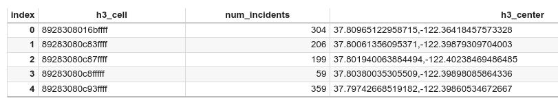
To compute the cell for each incident's latitude and longitude, aggregate the incidents for each cell, construct a
geopandasDataFrame, and add the center of each hexagon for the heatmap layer, enter the following code:# Compute the cell for each incident's latitude and longitude. H3_RESOLUTION = 9 gdf_incidents['h3_cell'] = gdf_incidents.geometry.apply( lambda geom: h3.latlng_to_cell(geom.y, geom.x, H3_RESOLUTION) ) # Aggregate the incidents for each hexagon cell. count_incidents = gdf_incidents.groupby(by='h3_cell')['unique_key'].count().rename('num_incidents') # Construct a new geopandas.GeoDataFrame with the aggregate results. # Add the center of each hexagon for the HeatmapLayer to render. gdf_incidents_x_cell = gpd.GeoDataFrame(data=count_incidents).reset_index() gdf_incidents_x_cell['h3_center'] = gdf_incidents_x_cell['h3_cell'].apply(h3.cell_to_latlng) gdf_incidents_x_cell.info()
Click Run cell.
The output is similar to the following:
<class 'geopandas.geodataframe.GeoDataFrame'>
RangeIndex: 969 entries, 0 to 968
Data columns (total 3 columns):
#   Column         Non-Null Count  Dtype
--  ------         --------------  -----
0   h3_cell        969 non-null    object
1   num_incidents  969 non-null    Int64
2   h3_center      969 non-null    object
dtypes: Int64(1), object(2)
memory usage: 23.8+ KB
To insert a code cell, click Code.
To preview the first five rows of the DataFrame, enter the following code:
# Preview the first five rows.
gdf_incidents_x_cell.head()
Click Run cell.
The output is similar to the following:
To insert a code cell, click Code.
To convert the data into a JSON format that can be used by
HeatmapLayer, enter the following code:# Convert to a JSON format recognized by the HeatmapLayer. def _make_heatmap_datum(row) -> dict: return { "latitude": row['h3_center'][0], "longitude": row['h3_center'][1], "weight": float(row['num_incidents']), } heatmap_data = gdf_incidents_x_cell.apply(_make_heatmap_datum, axis='columns').values.tolist()
Click Run cell.
After you run the code, no output is generated in your Colab notebook. The check mark beside the cell indicates that the code ran successfully.
To insert a code cell, click Code.
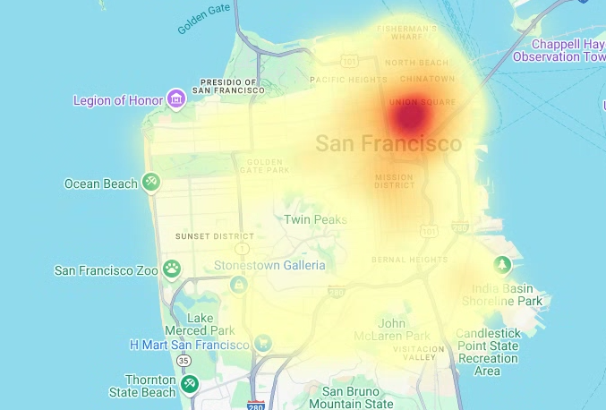
To render the heatmap, enter the following code:
# Render the heatmap.
heatmap_layer = pdk.Layer(
  "HeatmapLayer",
  id="sfpd_heatmap",
  data=heatmap_data,
  get_position=['longitude', 'latitude'],
  get_weight='weight',
  opacity=0.7,
  radius_pixels=99,  # this limitation can introduce artifacts (see above)
  aggregation='MEAN',
)
view_state = pdk.ViewState(latitude=37.77613, longitude=-122.42284, zoom=12)
display_pydeck_map([heatmap_layer], view_state)
Click Run cell.
The output is similar to the following:
Clean up
To avoid incurring charges to your Google Cloud account for the resources used in this tutorial, either delete the project that contains the resources, or keep the project and delete the individual resources.
Delete the project
Console
- In the Google Cloud console, go to the Manage resources page.
- In the project list, select the project that you want to delete, and then click Delete.
- In the dialog, type the project ID, and then click Shut down to delete the project.
gcloud
- In the Google Cloud console, go to the Manage resources page.
- In the project list, select the project that you want to delete, and then click Delete.
- In the dialog, type the project ID, and then click Shut down to delete the project.
Delete your Google Maps API key and notebook
After you delete the Google Cloud project, if you used the Google Maps API, delete the Google Maps API key from your Colab Secrets and then optionally delete the notebook.
In your Colab, click Secrets.
At the end of the
GMP_API_KEYrow, click Delete.Optional: To delete the notebook, click File > Move to trash.
What's next
- For more information on geospatial analytics in BigQuery, see Introduction to geospatial analytics in BigQuery.
- For an introduction to visualizing geospatial data in BigQuery, see Visualize geospatial data.
- To learn more about
pydeckand otherdeck.glchart types, you can find examples in thepydeckGallery, thedeck.glLayer Catalog, and thedeck.glGitHub source. - For more information on working with geospatial data in data frames, see the GeoPandas Getting started page and the GeoPandas User guide.
- For more information on geometric object manipulation, see the Shapely user manual.
- To explore using Google Earth Engine data in BigQuery, see Exporting to BigQuery in the Google Earth Engine documentation.