Best practices for spatial analysis
This document describes best practices for optimizing geospatial query performance in BigQuery. You can use these best practices to improve performance and reduce cost and latency.
Datasets can contain large collections of polygons, multipolygon shapes, and linestrings to represent complex features—for example, roads, land parcels, and flood zones. Each shape can contain thousands of points. In most spatial operations in BigQuery (for example, intersections and distance calculations), the underlying algorithm usually visits the majority of points in each shape to produce a result. For some operations, the algorithm visits all points. For complex shapes, visiting each point can increase the cost and duration of the spatial operations. You can use the strategies and methods presented in this guide to optimize these common spatial operations for improved performance and reduced cost.
This document assumes that your BigQuery geospatial tables are clustered on a geography column.
Simplify shapes
Best practice: Use simplify and snap-to-grid functions to store a simplified version of your original dataset as a materialized view.
Many complex shapes with large numbers of points can be simplified without much
loss in precision. Use the BigQuery
ST_SIMPLIFY and
ST_SNAPTOGRID
functions separately or together to reduce the number of points in complex shapes.
Combine these functions with BigQuery
materialized views to store a
simplified version of your original dataset as a materialized view that's
automatically kept up to date against the base table.
Simplifying shapes is most useful for improving the cost and performance of a dataset in the following use cases:
- You need to maintain a high degree of similarity to the true shape.
- You must perform high-precision, high-accuracy operations.
- You want to speed up visualizations without visible loss in shape detail.
The following code sample shows how to use the ST_SIMPLIFY function on a base
table that has a GEOGRAPHY column named geom. The code simplifies shapes
and removes points without disturbing any edge of a shape by more
than the given tolerance of 1.0 meters.
CREATE MATERIALIZED VIEW project.dataset.base_mv
  CLUSTER BY geom
AS (
  SELECT
    * EXCEPT (geom),
    ST_SIMPLIFY(geom, 1.0) AS geom
  FROM base_table
)
The following code sample shows how to use the ST_SNAPTOGRID function to snap
the points to a grid with a resolution of 0.00001 degrees:
CREATE MATERIALIZED VIEW project.dataset.base_mv
  CLUSTER BY geom
AS (
  SELECT
    * EXCEPT (geom),
    ST_SNAPTOGRID(geom, -5) AS geom
  FROM base_table
)
The grid_size argument in this function serves as the exponent, which means
10e-5 = 0.00001. This resolution is equivalent to around 1 meter in the worst
case, which occurs at the equator.
After you create these views, query the base_mv view using the same query
semantics you would use to query the base table. You can use this technique
to quickly identify a collection of shapes that need to be analyzed more deeply,
and then you can perform a second deeper analysis on the base table. Test your
queries to see which threshold values work best for your data.
For measurement use cases, determine the level of accuracy that your use case
requires. When using the ST_SIMPLIFY function, set the threshold_meters
parameter to the required level of accuracy. For measuring distances at the scale
of a city or larger, set a threshold of 10 meters. At smaller scales—for
example, when measuring the distance between a building and the nearest body of
water—consider using a smaller threshold of 1 meter or less. Using smaller
threshold values results in removing fewer points from the given shape.
When serving map layers from a web service, you can precalculate materialized
views for different zoom levels with the
bigquery-geotools project,
which is a driver for Geoserver that lets you serve spatial layers from
BigQuery. This driver creates multiple materialized views with
different ST_SIMPLIFY threshold parameters so that less detail is served at
higher zoom levels.
Use points and rectangles
Best practice: Reduce the shape to a point or rectangle to represent its location.
You can improve query performance by reducing the shape to a single point or a rectangle. The methods in this section don't accurately represent the details and proportions of the shape, but rather optimize for representing the location of the shape.
You can use the geographic central point of a shape (its centroid) to represent the location of the whole shape. Use a rectangle containing the shape to create the shape's extent, which you can use to represent the shape's location and maintain information about its relative size.
Using points and rectangles is most useful for improving the cost and performance of a dataset when you need to measure the distance between two points, such as between two cities.
For example, consider loading a database of land parcels in the United States into
a BigQuery table and then determining the nearest body of water.
In this case, precomputing parcel centroids using the
ST_CENTROID
function in combination with the method described in the
Simplify shapes section of this document can reduce the
number of comparisons performed when using the
ST_DISTANCE or
ST_DWITHIN
functions. When using the ST_CENTROID function, the parcel centroid needs to
be considered in the calculation. Precomputing the parcel centroids in this way
can also reduce variability in performance, because different parcel shapes are
likely to contain different numbers of points.
A variant of this method is to use the
ST_BOUNDINGBOX
function instead of the ST_CENTROID function to compute a rectangular envelope
around the input shape. While it's not quite as efficient as using a single point,
it can reduce the occurrence of certain edge cases. This variant still offers
good and consistent performance, since the output of the ST_BOUNDINGBOX
function always contains only four points that need to be considered. The
bounding box result will be of the type
STRUCT, which
means you'll need to calculate the distances manually or use the
vector index method described later in
this document.
Use hulls
Best practice: Use a hull to optimize for representing the location of a shape.
If you imagine shrink-wrapping a shape and computing the boundary of the shrink wrap, that boundary is called the hull. In a convex hull, all the angles of the resulting shape are convex. Like a shape's extent, a convex hull retains some information about the underlying shape's relative size and proportions. However, using a hull comes at the cost of needing to store and consider more points in subsequent analyses.
You can use the ST_CONVEXHULL function to optimize for representing the
location of the shape. Using this function improves accuracy, but this comes
at the cost of decreased performance. The ST_CONVEXHULL function is similar to
the ST_EXTENT
function, except the output shape contains more points and varies in the number
of points based on the complexity of the input shape. While the performance
benefit is likely negligible for small datasets of non-complex shapes, for very
large datasets with large and complex shapes, the ST_CONVEXHULL function offers
a good balance between cost, performance, and accuracy.
Use grid systems
Best practice: Use geospatial grid systems to compare areas.
If your use cases involve aggregating data within localized areas and comparing statistical aggregations of those areas with each other, you can benefit from utilizing a standardized grid system to compare different areas.
For example, a retailer might want to analyze demographic changes over time in areas where their stores are located or where they are contemplating building a new store. Or, an insurance company might want to improve their understanding of property risks by analyzing the prevailing natural hazard risks in a particular area.
Using standard grid systems such as S2 and H3 can speed up such statistical aggregations and spatial analyses. Using these grid systems can also simplify the development of analytics and improve development efficiency.
For example, comparisons using census tracts in the United States suffer from inconsistency in size, which means corrective factors need to be applied to perform like-for-like comparisons between census tracts. Additionally, census tracts and other administrative boundaries change over time and require effort to correct for these changes. Using grid systems for spatial analysis can address such challenges.
Use vector search and vector indexes
Best practice: Use vector search and vector indexes for nearest-neighbor geospatial queries.
Vector search capabilities were introduced in BigQuery to enable machine-learning use cases such as semantic search, similarity detection, and retrieval-augmented generation. The key to enabling these use cases is an indexing method called approximate nearest-neighbor search. You can use vector search to speed up and simplify nearest-neighbor geospatial queries by comparing vectors that represent points in space.
You can use vector search to search for features by radius. First, establish a
radius for your search. You can discover the optimal radius in the result set of
a nearest-neighbor search. After you establish the radius, use the
ST_DWITHIN
function to identify nearby features.
For example, consider finding the ten buildings nearest to a particular anchor building that you already have the location of. You can store the centroids of each building as a vector in a new table, index the table, and search using vector search.
For this example, you can also use
Overture Maps data in BigQuery
to create a separate table of building shapes corresponding to an area of
interest and a vector called geom_vector. The area of interest in this example
is the city of Norfolk, VA, United States, represented by
FIPS code
51710, as shown in the following code sample:
CREATE TABLE vector_search.norfolk_buildings
AS (
  SELECT
    *,
    [
      ST_X(ST_CENTROID(building.geometry)),
      ST_Y(ST_CENTROID(building.geometry))] AS geom_vector
  FROM `bigquery-public-data.overture_maps.building` AS building
  INNER JOIN `bigquery-public-data.geo_us_boundaries.counties` AS county
    ON (st_intersects(county.county_geom, building.geometry))
  WHERE county.county_fips_code = '51710'
)
The following code sample shows how to create a vector index on the table:
CREATE
  vector index building_vector_index
ON
  vector_search.norfolk_buildings(geom_vector)
  OPTIONS (index_type = 'IVF')
This query identifies the 10 buildings nearest to a particular anchor building:
SELECT base.*
FROM
  VECTOR_SEARCH(
    TABLE vector_search.norfolk_buildings,
    'geom_vector',
    (
      SELECT
        geom_vector
      FROM
        vector_search.norfolk_buildings
      WHERE id = '56873794-9873-4fe1-871a-5987bb3a0efb'
    ),
    top_k => 10,
    distance_type => 'EUCLIDEAN',
    options => '{"fraction_lists_to_search":0.1}')
In the Query results pane, click the Visualization tab. The map shows a cluster of building shapes nearest to the anchor building:
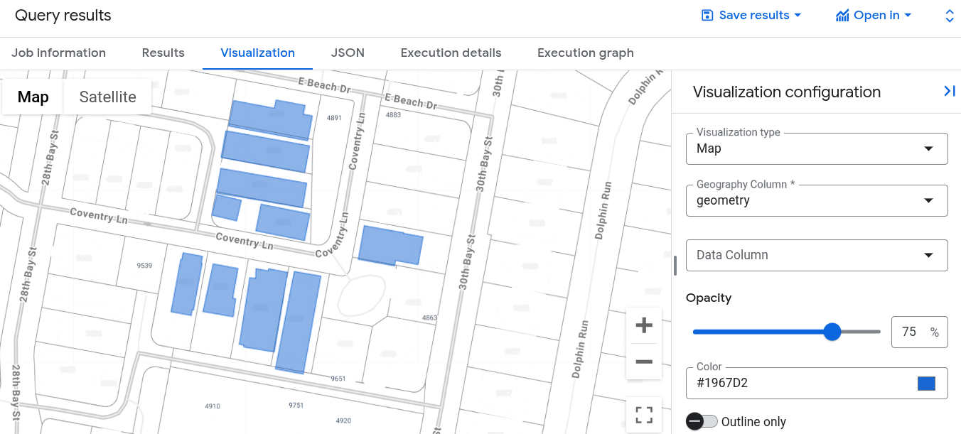
When you run this query in the Google Cloud console, click Job Information and
verify that Vector Index Usage Mode is set to FULLY_USED. This indicates
that the query is leveraging the building_vector_index vector index, which you
created earlier.
Divide large shapes
Best practice: Divide large shapes with the ST_SUBDIVIDE function.
Use the ST_SUBDIVIDE function to
break large shapes or long line strings into smaller shapes.
What's next
- Learn how to use grid systems for spatial analysis.
- Learn more about BigQuery geography functions.
- Learn how to manage vector indexes.
- Learn more about best practices for spatial indexing and clustering in BigQuery.
- For more information on analyzing and visualizing geospatial data in BigQuery, see Get started with geospatial analytics.