Grid systems for spatial analysis
This document explains the purpose and methods of using geospatial grid systems (such as S2 and H3) in BigQuery to organize spatial data in standardized geographic areas. It also explains how to choose the right grid system for your application. This document is useful for anyone who works with spatial data and performs spatial analysis in BigQuery.
Overview and challenges of using spatial analysis
Spatial analytics helps to show the relation between entities (shops or houses) and events in a physical space. Spatial analytics that use the surface of the earth as the physical space is called geospatial analytics. BigQuery includes geospatial features and functions that enable you to perform geospatial analysis at scale.
Many geospatial use cases involve aggregating data within localized areas, and comparing statistical aggregations of those areas with each other. These localized areas are represented as polygons in a spatial database table. In some contexts, this method is called statistical geography. The method of determining the extent of the geographic areas needs to be standardized for better reporting, analysis, and spatial indexing. For example, a retailer might want to analyze the changes in demographics over time in areas where their stores are located, or in areas where they are contemplating building a new store. Or, an insurance company might want to improve their understanding of property risks by analyzing prevailing natural hazard risks in a particular area.
Due to strict data privacy regulations in many areas, datasets that contain location information need to be de-identified or partially anonymized to help protect the privacy of individuals represented in the data. For example, you might need to perform a geographic credit concentration risk analysis on a dataset that contains data about outstanding mortgage loans. To de-identify the dataset to make it suitable for compliant analysis, you need to retain relevant information about the location of the properties, but avoid using a specific address or longitude and latitude coordinates.
In the preceding examples, the designers of these analyses are presented with the following challenges:
- How to draw the area boundaries within which you analyze changes over time?
- How to use the existing administrative boundaries such as census tracts or a multi-resolution grid system?
This document aims to answer these questions by explaining each option, describing best practices, and helping you avoid common pitfalls.
Common pitfalls while choosing statistical areas
Business datasets such as real estate sales, marketing campaigns, ecommerce shipments, and insurance policies are suitable for spatial analysis. Often these datasets contain what appears to be a convenient spatial join key, such as a census tract, a zip code, or the name of a city. Public datasets that contain representations of census tracts, zip codes, and cities are readily available, making them tempting to use as administrative boundaries for statistical aggregation.
While nominally convenient, these and other administrative boundaries come with drawbacks. Moreover, these boundaries might work well in the early stages of an analytics project, but the drawbacks can be noticed in the later stages.
Postal codes
Postal codes are used to route mail in various countries around the world, and due to this ubiquity, are often used to reference locations and areas in both spatial and non-spatial datasets. Referring to the preceding example about the mortgage loan, a dataset often needs to be de-identified before downstream analysis can be performed. Since each property address contains a zip code, zip code reference tables are accessible, making it a convenient option for a join key for spatial analysis.
A pitfall in using postal codes is that they are not represented as polygons, and there is no single correct source of truth for postal code areas. Additionally, postal codes are not a good representation of real human behavior. The most commonly used postal code data in the US is from the US Census Bureau TIGER/Line Shapefiles, which contains a dataset called ZCTA5 (Zip Code Tabulation Area). This dataset represents an approximation of zip code boundaries that are derived from mail delivery routes. However, some zip codes that represent individual buildings have no boundary at all. This problem is present in other countries as well, making it difficult to form a single global fact table that contains an authoritative set of postal code boundaries that can be used across systems and across datasets.
Additionally, there's no standardized postal code format used around the world. Some are numeric, ranging from three to ten digits, while some are alphanumeric. There is also an overlap between countries, making it necessary to store the country of origin in a separate column along with the postal code. Some countries don't use postal codes, further complicating the analysis.
Census tracts, cities, and counties
There are some administrative units, such as census tracts, cities, and counties that don't suffer from the lack of an authoritative boundary. The boundaries of cities, for example, are in most cases well established by government authorities. Census tracts are well-defined by the US Census Bureau, and by their analogous institutions in most other countries.
A drawback of using these and other administrative boundaries is that they change over time, and are not geographically consistent with one another. Counties and cities merge or break apart from one another and are occasionally renamed. Census tracts are updated once each decade in the US, and at different times in other countries. Confusingly, in some cases the geographic boundary can change but its unique identifier remains the same, making it difficult to analyze and understand changes over time.
Another drawback that is common to some administrative boundaries is that they are discrete areas with no geographic hierarchy. In addition to comparing individual areas with one another, a common requirement is to compare aggregations of the areas themselves to other aggregations. For example, a retailer implementing the Huff model might want to run this analysis using multiple distances, which might not correspond to administrative areas that are used elsewhere in the business.
Single and multi-resolution grids
Single-resolution grids consist of discrete units that have no geographic relation to larger areas that contain those units. For example, postal codes have an inconsistent geographic relationship with the boundaries of larger administrative units, such as cities or counties that might contain zip codes. For spatial analysis, it is important to understand how different areas are related to each other without deep knowledge of the history and legislation that defines the area polygon.
Multi-resolution grids are sometimes called hierarchical grids because cells at each zoom level are subdivided into smaller cells at higher zoom levels. Multi-resolution grids consist of a well-defined hierarchy of units that are contained within larger units. Census tracts, for example, contain block groups, which in turn contain blocks. This consistent hierarchical relationship can be useful for statistical aggregation. For example, by taking an average of incomes of all the block groups contained in a tract, you can show the average income for that census tract containing the block groups. This wouldn't be possible with postal codes because all postal areas are located at a single resolution. It would be difficult to compare the income of a tract with its surrounding tracts as there's no standardized way of defining adjacency, or comparing income in different countries.
S2 and H3 grid systems
This section provides an overview of S2 and H3 grid systems.
S2
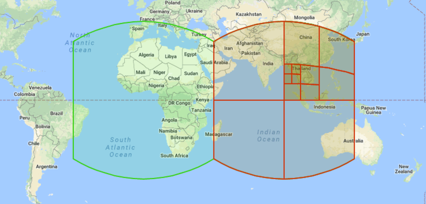
S2 geometry is an open source hierarchical grid system developed by Google and released to the public in 2011. You can use the S2 grid system to organize and index spatial data by assigning a unique 64-bit integer to each cell. There are 31 levels of resolution. Each cell is represented as a square and is designed for operations on spherical geometries (sometimes called geographies). Each square is subdivided into four smaller squares. Neighbor traversal, which is the ability to identify neighboring S2 cells, is less well-defined because squares can have either four or eight relevant neighbors depending on the type of analysis. The following is an example of multi-resolution S2 grid cells:
BigQuery uses S2 cells to index spatial data and exposes
multiple functions. For example, S2_CELLIDFROMPOINT
returns the S2 cell ID that contains a point on earth's surface at a given level.
H3
H3 is an open source hierarchical grid system developed by Uber and used by Overture Maps. There are 16 levels of resolution. Each cell is represented as a hexagon, and like S2, each cell is assigned a unique 64-bit integer. In the example about visualization of H3 cells covering the Gulf of Mexico, the smaller H3 cells are not perfectly contained by the larger cells.
Each cell subdivides into seven smaller hexagons. The subdivision isn't exact, but it is adequate for many use cases. Each cell shares an edge with six neighboring cells, simplifying neighbor traversal. For example, at each level, there are 12 pentagons, which instead share an edge with five neighbors instead of six. Although H3 is not supported in BigQuery, you can add H3 support to BigQuery using the Carto Analytics Toolbox for BigQuery.
While both S2 and H3 libraries are open source and available under the Apache 2 license, the H3 library has more detailed documentation.
HEALPix
An additional scheme to grid the sphere, commonly used in the astronomy field, is known as Hierarchical Equal Area isoLatitude Pixelation (HEALPix). HEALPix is independent of hierarchical pixel depth, but the compute time remains constant.
HEALPix is a hierarchical equal-area pixelization scheme for the sphere. It is used to represent and analyze data on the celestial (or other) sphere. In addition to constant compute time, the HEALPix grid has the following characteristics:
- The grid cells are hierarchical, where parent-child relationships are maintained.
- At a specific hierarchy, cells are of equal areas.
- The cells follow an iso-latitude distribution, allowing higher performance for spectral methods.
BigQuery does not support HEALPix, but there are numerous implementations across a variety of languages, including JavaScript, which makes it convenient for use in BigQuery user-defined functions (UDFs).
Example use cases for each indexing strategy
This section provides some examples that help you evaluate which is the best grid system for your use case.
Many analytics and reporting use cases involve visualization, either as part of the analysis itself or for reporting to business stakeholders. These visualizations are commonly presented in Web Mercator, which is the planar projection that is used by Google Maps and many other web mapping applications. In cases where visualization plays a vital role, H3 cells deliver a subjectively better visualization experience. S2 cells, especially at higher latitudes, tend to appear more distorted than H3, and don't appear consistent with cells of lower latitudes when presented in a planar projection.
H3 cells simplify implementation where neighbor comparison plays an important role in the analysis. For example, a comparative analysis between sections of a city might help to decide which location is suitable for opening a new retail store or distribution center. The analysis requires statistical calculations for attributes of a given cell that is compared with its neighboring cells.
S2 cells can work better in analyses that are global in nature, such as analyses that involve measurements of distances and angles. Pokemon Go by Niantic utilizes S2 cells to determine where game assets are placed and how they are distributed. The exact subdivision property of S2 cells ensures that game assets can be evenly distributed across the globe.
What's next
- For best practices for spatial clustering, see Spatial Clustering on BigQuery - Best Practices.
- Learn to create a spatial hierarchy from imperfect data.
- Learn about S2 geometry on GitHub.
- Learn about H3 geometry on GitHub.
- See examples that use H3, BigQuery, and Earth Engine.