In this tutorial, you will learn how to significantly accelerate training of
a set of
ARIMA_PLUS univariate time series model,
in order to perform multiple time-series forecasts with a single
query. You will also learn how to evaluate forecasting accuracy.
This tutorial forecasts for multiple time series. Forecasted values are calculated for each time point, for each value in one or more specified columns. For example, if you wanted to forecast weather and specified a column containing city data, the forecasted data would contain forecasts for all time points for City A, then forecasted values for all time points for City B, and so forth.
This tutorial uses data from the public
bigquery-public-data.new_york.citibike_trips
and
iowa_liquor_sales.sales
tables. The bike trips data only contains a few hundred time series, so it is
used to illustrate various strategies to accelerate model training.
The liquor sales data has more than 1 million time series, so it is used to show
time series forecasting at scale.
Before reading this tutorial, you should read Forecast multiple time series with a univariate model and Large-scale time series forecasting best practices.
Objectives
In this tutorial, you use the following:
- Creating a time series model by using the
CREATE MODELstatement. - Evaluating the model's accuracy by using the
ML.EVALUATEfunction. - Using the
AUTO_ARIMA_MAX_ORDER,TIME_SERIES_LENGTH_FRACTION,MIN_TIME_SERIES_LENGTH, andMAX_TIME_SERIES_LENGTHoptions of theCREATE MODELstatament to significantly reduce the model training time.
For simplicity, this tutorial doesn't cover how to use the
ML.FORECAST
or
ML.EXPLAIN_FORECAST
functions to generate forecasts. To learn how to use those functions, see
Forecast multiple time series with a univariate model.
Costs
This tutorial uses billable components of Google Cloud, including:
- BigQuery
- BigQuery ML
For more information about costs, see the BigQuery pricing page and the BigQuery ML pricing page.
Before you begin
- Sign in to your Google Cloud account. If you're new to Google Cloud, create an account to evaluate how our products perform in real-world scenarios. New customers also get $300 in free credits to run, test, and deploy workloads.
-
In the Google Cloud console, on the project selector page, select or create a Google Cloud project.
Roles required to select or create a project
- Select a project: Selecting a project doesn't require a specific IAM role—you can select any project that you've been granted a role on.
-
Create a project: To create a project, you need the Project Creator
(
roles/resourcemanager.projectCreator), which contains theresourcemanager.projects.createpermission. Learn how to grant roles.
-
Verify that billing is enabled for your Google Cloud project.
-
In the Google Cloud console, on the project selector page, select or create a Google Cloud project.
Roles required to select or create a project
- Select a project: Selecting a project doesn't require a specific IAM role—you can select any project that you've been granted a role on.
-
Create a project: To create a project, you need the Project Creator
(
roles/resourcemanager.projectCreator), which contains theresourcemanager.projects.createpermission. Learn how to grant roles.
-
Verify that billing is enabled for your Google Cloud project.
- BigQuery is automatically enabled in new projects.
To activate BigQuery in a pre-existing project, go to
Enable the BigQuery API.
Roles required to enable APIs
To enable APIs, you need the Service Usage Admin IAM role (
roles/serviceusage.serviceUsageAdmin), which contains theserviceusage.services.enablepermission. Learn how to grant roles.
Required Permissions
To create the dataset, you need the
bigquery.datasets.createIAM permission.To create the model, you need the following permissions:
bigquery.jobs.createbigquery.models.createbigquery.models.getDatabigquery.models.updateData
To run inference, you need the following permissions:
bigquery.models.getDatabigquery.jobs.create
For more information about IAM roles and permissions in BigQuery, see Introduction to IAM.
Create a dataset
Create a BigQuery dataset to store your ML model.
Console
In the Google Cloud console, go to the BigQuery page.
In the Explorer pane, click your project name.
Click View actions > Create dataset
On the Create dataset page, do the following:
For Dataset ID, enter
bqml_tutorial.For Location type, select Multi-region, and then select US (multiple regions in United States).
Leave the remaining default settings as they are, and click Create dataset.
bq
To create a new dataset, use the
bq mk command
with the --location flag. For a full list of possible parameters, see the
bq mk --dataset command
reference.
Create a dataset named
bqml_tutorialwith the data location set toUSand a description ofBigQuery ML tutorial dataset:bq --location=US mk -d \ --description "BigQuery ML tutorial dataset." \ bqml_tutorial
Instead of using the
--datasetflag, the command uses the-dshortcut. If you omit-dand--dataset, the command defaults to creating a dataset.Confirm that the dataset was created:
bq ls
API
Call the datasets.insert
method with a defined dataset resource.
{
  "datasetReference": {
     "datasetId": "bqml_tutorial"
  }
}
BigQuery DataFrames
Before trying this sample, follow the BigQuery DataFrames setup instructions in the BigQuery quickstart using BigQuery DataFrames. For more information, see the BigQuery DataFrames reference documentation.
To authenticate to BigQuery, set up Application Default Credentials. For more information, see Set up ADC for a local development environment.
Create a table of input data
The SELECT statement of the following query uses the
EXTRACT function
to extract the date information from the starttime column. The query uses
the COUNT(*) clause to get the daily total number of Citi Bike trips.
table_1 has 679 time series. The query uses additional INNER JOIN logic
to select all those time series that have more than 400 time points, resulting
in a total of 383 times series.
Follow these steps to create the input data table:
In the Google Cloud console, go to the BigQuery page.
In the query editor, paste in the following query and click Run:
CREATE OR REPLACE TABLE
  `bqml_tutorial.nyc_citibike_time_series` AS
WITH input_time_series AS
(
  SELECT
    start_station_name,
    EXTRACT(DATE FROM starttime) AS date,
    COUNT(*) AS num_trips
  FROM
    `bigquery-public-data.new_york.citibike_trips`
  GROUP BY
    start_station_name, date
)
SELECT table_1.*
FROM input_time_series AS table_1
INNER JOIN (
  SELECT start_station_name,  COUNT(*) AS num_points
  FROM input_time_series
  GROUP BY start_station_name) table_2
ON
  table_1.start_station_name = table_2.start_station_name
WHERE
  num_points > 400;
Create a model to multiple time-series with default parameters
You want to forecast the number of bike trips for each
Citi Bike station, which requires many time series models; one for each
Citi Bike station that is included in the input data. You can write multiple
CREATE MODEL
queries to do this, but that can be a tedious and time consuming process,
especially when you have a large number of time series. Instead, you can use a
single query to create and fit a set of time series models in order to forecast
multiple time series at once.
The OPTIONS(model_type='ARIMA_PLUS', time_series_timestamp_col='date', ...)
clause indicates that you are creating a set of
ARIMA-based time-series ARIMA_PLUS models. The
time_series_timestamp_col option specifies the column that contains the times
series, the time_series_data_col option specifies the column to forecast for,
and the time_series_id_colspecifies one or more dimensions that you want to
create time series for.
This example leaves out the time points in the time series after Jun1 , 2016
so that those time points can be used to evaluate the forecasting accuracy
later by using the ML.EVALUATE function.
Follow these steps to create the model:
In the Google Cloud console, go to the BigQuery page.
In the query editor, paste in the following query and click Run:
CREATE OR REPLACE MODEL `bqml_tutorial.nyc_citibike_arima_model_default`
OPTIONS
  (model_type = 'ARIMA_PLUS',
  time_series_timestamp_col = 'date',
  time_series_data_col = 'num_trips',
  time_series_id_col = 'start_station_name'
  ) AS
SELECT *
FROM bqml_tutorial.nyc_citibike_time_series
WHERE date < '2016-06-01';
The query takes about 15 minutes to complete.
Evaluate forecasting accuracy for each time series
Evaluate the forecasting accuracy of the model by using the ML.EVALUATE
function.
Follow these steps to evaluate the model:
In the Google Cloud console, go to the BigQuery page.
In the query editor, paste in the following query and click Run:
SELECT *
FROM
  ML.EVALUATE(MODEL `bqml_tutorial.nyc_citibike_arima_model_default`,
  TABLE `bqml_tutorial.nyc_citibike_time_series`,
  STRUCT(7 AS horizon, TRUE AS perform_aggregation));
This query reports several forecasting metrics, including:
The results should look similar to the following:
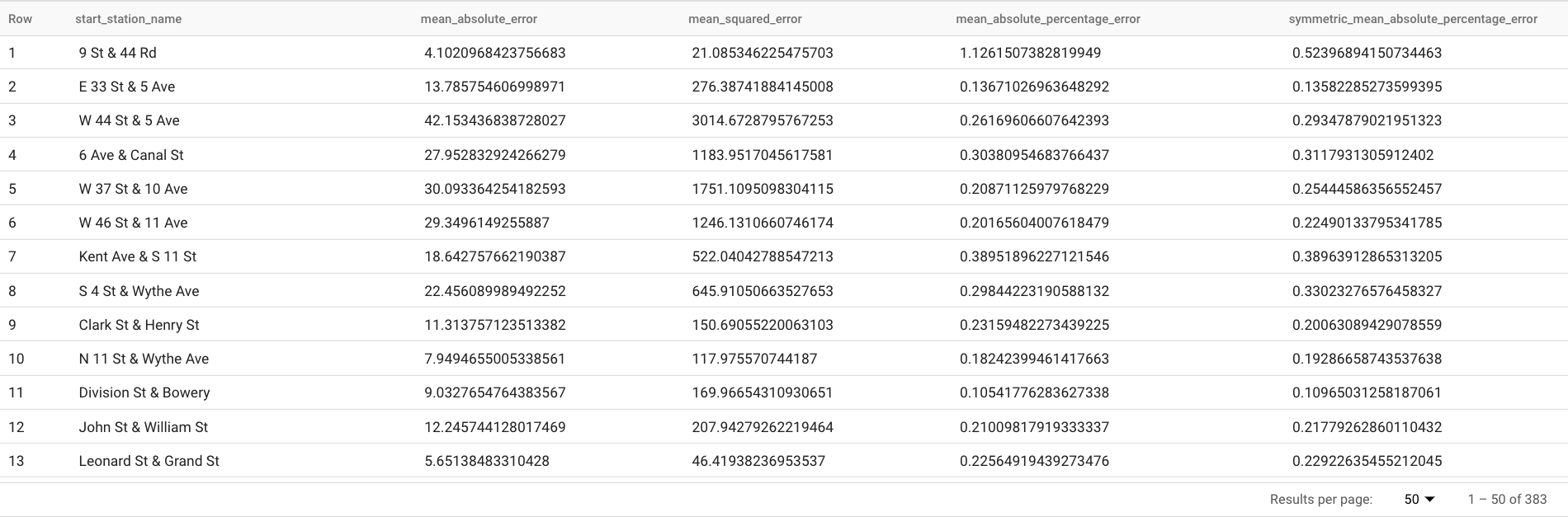
The
TABLEclause in theML.EVALUATEfunction identifies a table containing the ground truth data. The forecasting results are compared to the ground truth data to compute accuracy metrics. In this case, thenyc_citibike_time_seriescontains both the time series points that are before and after June 1, 2016. The points after June 1, 2016 are the ground truth data. The points before June 1, 2016 are used to train the model to generate forecasts after that date. Only the points after June 1, 2016 are necessary to compute the metrics. The points before June 1, 2016 are ignored in metrics calculation.The
STRUCTclause in theML.EVALUATEfunction specified parameters for the function. Thehorizonvalue is7, which means the query is calculating the forecasting accuracy based on a seven point forecast. Note that if the ground truth data has less than seven points for the comparison, then accuracy metrics are computed based on the available points only. Theperform_aggregationvalue isTRUE, which means that the forecasting accuracy metrics are aggregated over the metrics on the time point basis. If you specify aperform_aggregationvalue ofFALSE, forecasting accuracy is returned for each forecasted time point.For more information about the output columns, see
ML.EVALUATEfunction.
Evaluate overall forecasting accuracy
Evaluate the forecasting accuracy for the all 383 time series.
Of the forecasting metrics returned by ML.EVALUATE, only
mean absolute percentage error and symmetric mean absolute percentage error are
time series value independent. Therefore, to evaluate the entire forecasting accuracy of the set of time series, only the aggregate of these two metrics is meaningful.
Follow these steps to evaluate the model:
In the Google Cloud console, go to the BigQuery page.
In the query editor, paste in the following query and click Run:
SELECT
  AVG(mean_absolute_percentage_error) AS MAPE,
  AVG(symmetric_mean_absolute_percentage_error) AS sMAPE
FROM
  ML.EVALUATE(MODEL `bqml_tutorial.nyc_citibike_arima_model_default`,
    TABLE `bqml_tutorial.nyc_citibike_time_series`,
    STRUCT(7 AS horizon, TRUE AS perform_aggregation));
This query returns a MAPE value of 0.3471, and a sMAPE value of 0.2563.
Create a model to forecast multiple time-series with a smaller hyperparameter search space
In the
Create a model to multiple time-series with default parameters
section, you used the default values for all of the training options, including
the auto_arima_max_orderoption. This option controls the search space
for hyperparameter tuning in the auto.ARIMA algorithm.
In the model created by the following query, you use a smaller search space
for the hyperparameters by changing the auto_arima_max_order option value
from the default of 5 to 2.
Follow these steps to evaluate the model:
In the Google Cloud console, go to the BigQuery page.
In the query editor, paste in the following query and click Run:
CREATE OR REPLACE MODEL `bqml_tutorial.nyc_citibike_arima_model_max_order_2`
OPTIONS
  (model_type = 'ARIMA_PLUS',
  time_series_timestamp_col = 'date',
  time_series_data_col = 'num_trips',
  time_series_id_col = 'start_station_name',
  auto_arima_max_order = 2
  ) AS
SELECT *
FROM `bqml_tutorial.nyc_citibike_time_series`
WHERE date < '2016-06-01';
The query takes about 2 minutes to complete. Recall that the previous model took about 15 minutes to complete when the
auto_arima_max_ordervalue was5, so this change improves model training speed gain by around 7x. If you wonder why the speed gain is not5/2=2.5x, this is because when theauto_arima_max_ordervalue increases, not only do the number of candidate models increase, but also the complexity. This causes the training time of the model increases.
Evaluate forecasting accuracy for a model with a smaller hyperparameter search space
Follow these steps to evaluate the model:
In the Google Cloud console, go to the BigQuery page.
In the query editor, paste in the following query and click Run:
SELECT
  AVG(mean_absolute_percentage_error) AS MAPE,
  AVG(symmetric_mean_absolute_percentage_error) AS sMAPE
FROM
  ML.EVALUATE(MODEL `bqml_tutorial.nyc_citibike_arima_model_max_order_2`,
    TABLE `bqml_tutorial.nyc_citibike_time_series`,
    STRUCT(7 AS horizon, TRUE AS perform_aggregation));
This query returns a MAPE value of 0.3337, and a sMAPE value of 0.2337.
In the
Evaluate overall forecasting accuracy
section, you evaluated a model with a larger hyperparameter search space,
where the auto_arima_max_order option value is 5. This resulted in a MAPE
value of 0.3471, and a sMAPE value of 0.2563. In this case, you can see
that a smaller hyperparameter search space actually gives higher forecasting
accuracy. One reason for this is that the auto.ARIMA algorithm only performs
hyperparameter tuning for the trend module of the entire modeling pipeline. The
best ARIMA model selected by the auto.ARIMA algorithm might not generate the
best forecasting results for the entire pipeline.
Create a model to forecast multiple time-series with a smaller hyperparameter search space and smart fast training strategies
In this step, you use both a smaller hyperparameter search space and the
smart fast training strategy by using one or more of the max_time_series_length,
max_time_series_length, or time_series_length_fraction training options.
While periodic modeling such as seasonality requires a certain number of time points, trend modeling requires fewer time points. Meanwhile, trend modeling is much more computationally expensive than other time series components such as seasonality. By using the fast training options above, you can efficiently model the trend component with a subset of the time series, while the other time series components use the entire time series.
The following example uses the max_time_series_length option to achieve fast
training. By setting the max_time_series_length option value to 30, only the
30 most recent time points are used to model the trend component. All 383
time series are still used to model the non-trend components.
Follow these steps to create the model:
In the Google Cloud console, go to the BigQuery page.
In the query editor, paste in the following query and click Run:
CREATE OR REPLACE MODEL `bqml_tutorial.nyc_citibike_arima_model_max_order_2_fast_training`
OPTIONS
  (model_type = 'ARIMA_PLUS',
  time_series_timestamp_col = 'date',
  time_series_data_col = 'num_trips',
  time_series_id_col = 'start_station_name',
  auto_arima_max_order = 2,
  max_time_series_length = 30
  ) AS
SELECT *
FROM `bqml_tutorial.nyc_citibike_time_series`
WHERE date < '2016-06-01';
The query takes about 35 seconds to complete. This is 3x faster compared to the query you used In the Create a model to forecast multiple time-series with a smaller hyperparameter search space section. Due to the constant time overhead for the non-training part of the query, such as data preprocessing, the speed gain is much higher when the number of time series is much larger than in this example. For a million time series, the speed gain approaches the ratio of the time series length and the value of the
max_time_series_lengthoption value. In that case, the speed gain is greater than 10x.
Evaluate forecasting accuracy for a model with a smaller hyperparameter search space and smart fast training strategies
Follow these steps to evaluate the model:
In the Google Cloud console, go to the BigQuery page.
In the query editor, paste in the following query and click Run:
SELECT
  AVG(mean_absolute_percentage_error) AS MAPE,
  AVG(symmetric_mean_absolute_percentage_error) AS sMAPE
FROM
  ML.EVALUATE(MODEL `bqml_tutorial.nyc_citibike_arima_model_max_order_2_fast_training`,
    TABLE `bqml_tutorial.nyc_citibike_time_series`,
    STRUCT(7 AS horizon, TRUE AS perform_aggregation));
This query returns a MAPE value of 0.3515, and a sMAPE value of 0.2473.
Recall that without the use of fast training strategies, the forecasting
accuracy results in a MAPE value of 0.3337 and a sMAPE value of 0.2337.
The difference between the two sets of metric values are within 3%, which is
statistically insignificant.
In short, you have used a smaller hyperparameter search space and smart fast
training strategies to make your model training more than 20x faster without
sacrificing forecasting accuracy. As mentioned earlier, with more time series,
the speed gain by the smart fast training strategies can be significantly
higher. Additionally, the underlying ARIMA library used by ARIMA_PLUS models
has been optimized to run 5x faster than before. Together, these gains enable
the forecasting of millions of time series within hours.
Create a model to forecast a million time series
In this step, you forecast liquor sales for over 1 million liquor products in different stores using the public Iowa liquor sales data. The model training uses a small hyperparameter search space as well as the smart fast training strategy.
Follow these steps to evaluate the model:
In the Google Cloud console, go to the BigQuery page.
In the query editor, paste in the following query and click Run:
CREATE OR REPLACE MODEL
  `bqml_tutorial.liquor_forecast_by_product`
OPTIONS(
  MODEL_TYPE = 'ARIMA_PLUS',
  TIME_SERIES_TIMESTAMP_COL = 'date',
  TIME_SERIES_DATA_COL = 'total_bottles_sold',
  TIME_SERIES_ID_COL = ['store_number', 'item_description'],
  HOLIDAY_REGION = 'US',
  AUTO_ARIMA_MAX_ORDER = 2,
  MAX_TIME_SERIES_LENGTH = 30
) AS
SELECT
  store_number,
  item_description,
  date,
  SUM(bottles_sold) as total_bottles_sold
FROM
  `bigquery-public-data.iowa_liquor_sales.sales`
WHERE date BETWEEN DATE("2015-01-01") AND DATE("2021-12-31")
GROUP BY store_number, item_description, date;
The query takes about 1 hour 16 minutes to complete.
Clean up
To avoid incurring charges to your Google Cloud account for the resources used in this tutorial, either delete the project that contains the resources, or keep the project and delete the individual resources.
- You can delete the project you created.
- Or you can keep the project and delete the dataset.
Delete your dataset
Deleting your project removes all datasets and all tables in the project. If you prefer to reuse the project, you can delete the dataset you created in this tutorial:
If necessary, open the BigQuery page in the Google Cloud console.
In the navigation, click the bqml_tutorial dataset you created.
Click Delete dataset to delete the dataset, the table, and all of the data.
In the Delete dataset dialog, confirm the delete command by typing the name of your dataset (
bqml_tutorial) and then click Delete.
Delete your project
To delete the project:
- In the Google Cloud console, go to the Manage resources page.
- In the project list, select the project that you want to delete, and then click Delete.
- In the dialog, type the project ID, and then click Shut down to delete the project.
What's next
- Learn how to forecast a single time series with a univariate model
- Learn how to forecast a single time series with a multivariate model
- Learn how to forecast multiple time series with a univariate model
- Learn how to hierarchically forecast multiple time series with a univariate model
- For an overview of BigQuery ML, see Introduction to AI and ML in BigQuery.