This tutorial teaches you how to use a k-means model in BigQuery ML to identify clusters in a set of data.
The k-means algorithm that groups your data into clusters is a form of unsupervised machine learning. Unlike supervised machine learning, which is about predictive analytics, unsupervised machine learning is about descriptive analytics. Unsupervised machine learning can help you understand your data so that you can make data-driven decisions.
The queries in this tutorial use geography functions available in geospatial analytics. For more information, see Introduction to geospatial analytics.
This tutorial uses the London Bicycle Hires public dataset. The data includes start and stop timestamps, station names, and ride duration.
Objectives
This tutorial guides you through completing the following tasks:- Examine the data used to train the model.
- Create a k-means clustering model.
- Interpret the data clusters produced, using BigQuery ML's visualization of the clusters.
- Run the
ML.PREDICTfunction on the k-means model to predict the likely cluster for a set of bike hire stations.
Costs
This tutorial uses billable components of Google Cloud, including the following:
- BigQuery
- BigQuery ML
For information on BigQuery costs, see the BigQuery pricing page.
For information on BigQuery ML costs, see BigQuery ML pricing.
Before you begin
- Sign in to your Google Cloud account. If you're new to Google Cloud, create an account to evaluate how our products perform in real-world scenarios. New customers also get $300 in free credits to run, test, and deploy workloads.
-
In the Google Cloud console, on the project selector page, select or create a Google Cloud project.
Roles required to select or create a project
- Select a project: Selecting a project doesn't require a specific IAM role—you can select any project that you've been granted a role on.
-
Create a project: To create a project, you need the Project Creator
(
roles/resourcemanager.projectCreator), which contains theresourcemanager.projects.createpermission. Learn how to grant roles.
-
Verify that billing is enabled for your Google Cloud project.
-
In the Google Cloud console, on the project selector page, select or create a Google Cloud project.
Roles required to select or create a project
- Select a project: Selecting a project doesn't require a specific IAM role—you can select any project that you've been granted a role on.
-
Create a project: To create a project, you need the Project Creator
(
roles/resourcemanager.projectCreator), which contains theresourcemanager.projects.createpermission. Learn how to grant roles.
-
Verify that billing is enabled for your Google Cloud project.
- BigQuery is automatically enabled in new projects.
To activate BigQuery in a pre-existing project, go to
Enable the BigQuery API.
Roles required to enable APIs
To enable APIs, you need the Service Usage Admin IAM role (
roles/serviceusage.serviceUsageAdmin), which contains theserviceusage.services.enablepermission. Learn how to grant roles.
Required Permissions
To create the dataset, you need the
bigquery.datasets.createIAM permission.To create the model, you need the following permissions:
bigquery.jobs.createbigquery.models.createbigquery.models.getDatabigquery.models.updateData
To run inference, you need the following permissions:
bigquery.models.getDatabigquery.jobs.create
For more information about IAM roles and permissions in BigQuery, see Introduction to IAM.
Create a dataset
Create a BigQuery dataset to store your k-means model:
In the Google Cloud console, go to the BigQuery page.
In the Explorer pane, click your project name.
Click View actions > Create dataset.

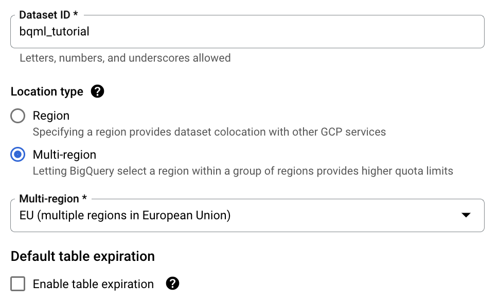
On the Create dataset page, do the following:
For Dataset ID, enter
bqml_tutorial.For Location type, select Multi-region, and then select EU (multiple regions in European Union).
The London Bicycle Hires public dataset is stored in the
EUmulti-region. Your dataset must be in the same location.Leave the remaining default settings as they are, and click Create dataset.

Examine the training data
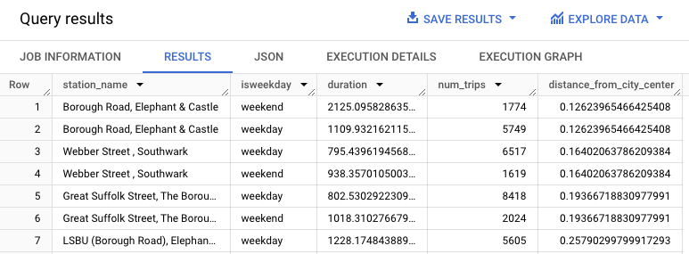
Examine the data you will use to train your k-means model. In this tutorial, you cluster bike stations based on the following attributes:
- Duration of rentals
- Number of trips per day
- Distance from city center
SQL
This query extracts data on cycle hires, including the start_station_name
and duration columns, and joins this data with station information. This
includes creating a calculated column that contains the station distance
from the city center. Then, it computes attributes of
the station in a stationstats column, including the average duration of
rides and the number of trips, and the calculated distance_from_city_center
column.
Follow these steps to examine the training data:
In the Google Cloud console, go to the BigQuery page.
In the query editor, paste in the following query and click Run:
WITH
hs AS (
  SELECT
    h.start_station_name AS station_name,
    IF(
      EXTRACT(DAYOFWEEK FROM h.start_date) = 1
        OR EXTRACT(DAYOFWEEK FROM h.start_date) = 7,
      'weekend',
      'weekday') AS isweekday,
    h.duration,
    ST_DISTANCE(ST_GEOGPOINT(s.longitude, s.latitude), ST_GEOGPOINT(-0.1, 51.5)) / 1000
      AS distance_from_city_center
  FROM
    `bigquery-public-data.london_bicycles.cycle_hire` AS h
  JOIN
    `bigquery-public-data.london_bicycles.cycle_stations` AS s
    ON
      h.start_station_id = s.id
  WHERE
    h.start_date
    BETWEEN CAST('2015-01-01 00:00:00' AS TIMESTAMP)
    AND CAST('2016-01-01 00:00:00' AS TIMESTAMP)
),
stationstats AS (
  SELECT
    station_name,
    isweekday,
    AVG(duration) AS duration,
    COUNT(duration) AS num_trips,
    MAX(distance_from_city_center) AS distance_from_city_center
  FROM
    hs
  GROUP BY
    station_name, isweekday
)
SELECT *
FROM
stationstats
ORDER BY
distance_from_city_center ASC;
The results should look similar to the following:

BigQuery DataFrames
Before trying this sample, follow the BigQuery DataFrames setup instructions in the BigQuery quickstart using BigQuery DataFrames. For more information, see the BigQuery DataFrames reference documentation.
To authenticate to BigQuery, set up Application Default Credentials. For more information, see Set up ADC for a local development environment.
Create a k-means model
Create a k-means model using London Bicycle Hires training data.
SQL
In the following query, the CREATE MODEL statement specifies the number of
clusters to use — four. In the SELECT statement, the EXCEPT clause
excludes the station_name column because this column doesn't contain a
feature. The query creates a unique row per station_name, and only the
features are mentioned in the SELECT statement.
Follow these steps to create a k-means model:
In the Google Cloud console, go to the BigQuery page.
In the query editor, paste in the following query and click Run:
CREATE OR REPLACE MODEL `bqml_tutorial.london_station_clusters`
OPTIONS (
  model_type = 'kmeans',
  num_clusters = 4)
AS
WITH
hs AS (
  SELECT
    h.start_station_name AS station_name,
    IF(
      EXTRACT(DAYOFWEEK FROM h.start_date) = 1
        OR EXTRACT(DAYOFWEEK FROM h.start_date) = 7,
      'weekend',
      'weekday') AS isweekday,
    h.duration,
    ST_DISTANCE(ST_GEOGPOINT(s.longitude, s.latitude), ST_GEOGPOINT(-0.1, 51.5)) / 1000
      AS distance_from_city_center
  FROM
    `bigquery-public-data.london_bicycles.cycle_hire` AS h
  JOIN
    `bigquery-public-data.london_bicycles.cycle_stations` AS s
    ON
      h.start_station_id = s.id
  WHERE
    h.start_date
    BETWEEN CAST('2015-01-01 00:00:00' AS TIMESTAMP)
    AND CAST('2016-01-01 00:00:00' AS TIMESTAMP)
),
stationstats AS (
  SELECT
    station_name,
    isweekday,
    AVG(duration) AS duration,
    COUNT(duration) AS num_trips,
    MAX(distance_from_city_center) AS distance_from_city_center
  FROM
    hs
  GROUP BY
    station_name, isweekday
)
SELECT *
EXCEPT (station_name, isweekday)
FROM
stationstats;
BigQuery DataFrames
Before trying this sample, follow the BigQuery DataFrames setup instructions in the BigQuery quickstart using BigQuery DataFrames. For more information, see the BigQuery DataFrames reference documentation.
To authenticate to BigQuery, set up Application Default Credentials. For more information, see Set up ADC for a local development environment.
Interpret the data clusters
The information in the models's Evaluation tab can help you to interpret the clusters produced by the model.
Follow these steps to view the model's evaluation information:
In the Google Cloud console, go to the BigQuery page.
In the Explorer pane, expand your project, expand the
bqml_tutorialdataset, and then expand the Models folder.Select the
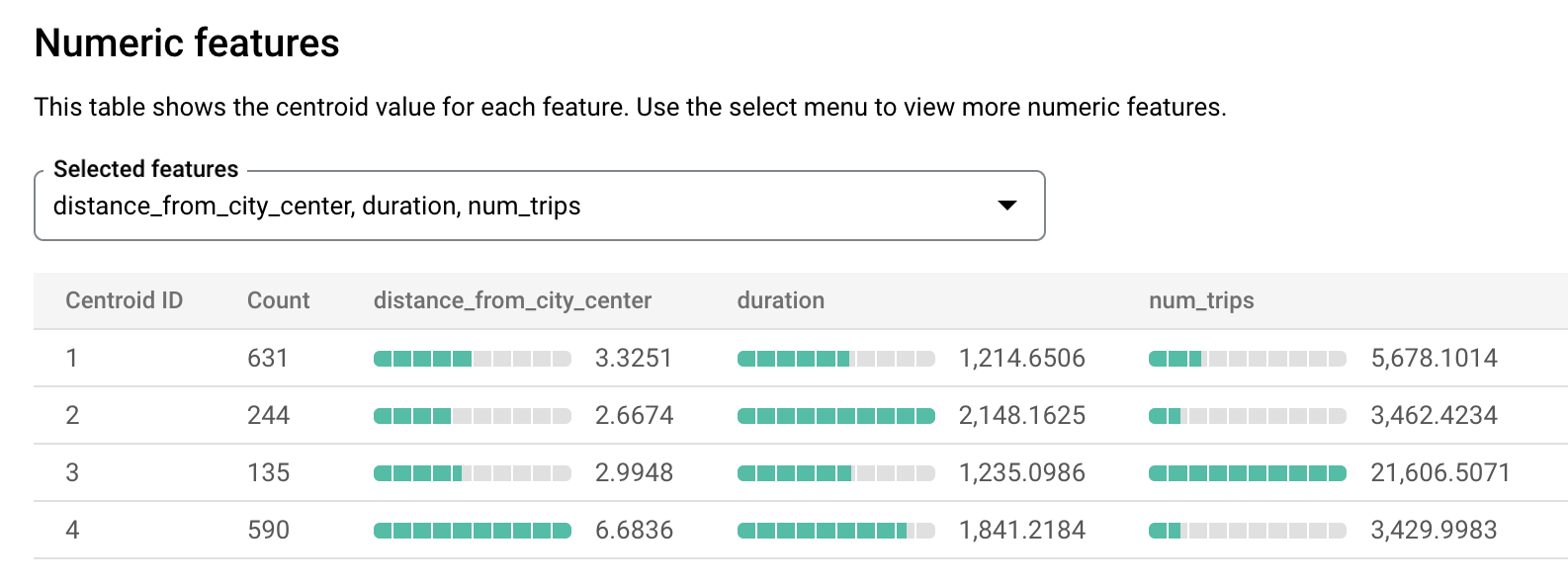
london_station_clustersmodel.Select the Evaluation tab. This tab displays visualizations of the clusters identified by the k-means model. In the Numeric features section, bar graphs display the most important numeric feature values for each centroid. Each centroid represents a given cluster of data. You can select which features to visualize from the drop-down menu.

This model creates the following centroids:
- Centroid 1 shows a less busy city station, with shorter duration rentals.
- Centroid 2 shows the second city station which is less busy and used for longer duration rentals.
- Centroid 3 shows a busy city station that is close to the city center.
- Centroid 4 shows a suburban station with trips that are longer.
If you were running the bicycle hire business, you could use this information to inform business decisions. For example:
Assume that you need to experiment with a new type of lock. Which cluster of stations should you choose as a subject for this experiment? The stations in centroid 1, centroid 2 or centroid 4 seem like logical choices because they are not the busiest stations.
Assume that you want to stock some stations with racing bikes. Which stations should you choose? Centroid 4 is the group of stations that are far from the city center, and they have the longest trips. These are likely candidates for racing bikes.
Use the ML.PREDICT function to predict a station's cluster
Identify the cluster to which a particular station belongs by using the
ML.PREDICT SQL function or the
predict BigQuery DataFrames function.
SQL
The following query uses the
REGEXP_CONTAINS
function to find all entries in the station_name column that contain the
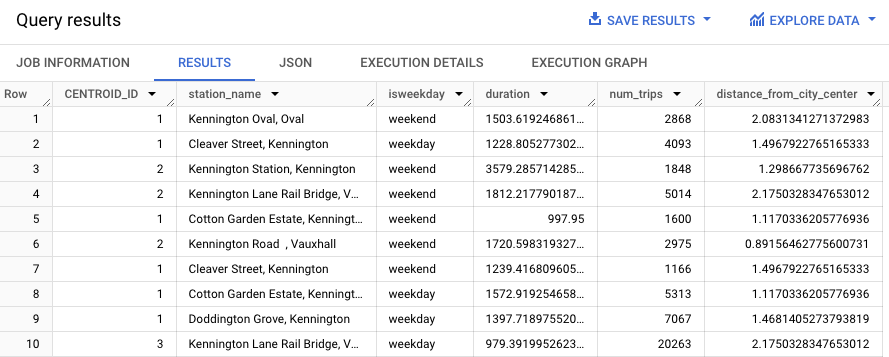
string Kennington. The ML.PREDICT function uses those values to predict
which clusters might contain those stations.
Follow these steps to predicts the cluster of every station that has
the string Kennington in its name:
In the Google Cloud console, go to the BigQuery page.
In the query editor, paste in the following query and click Run:
WITH
hs AS (
  SELECT
    h.start_station_name AS station_name,
    IF(
      EXTRACT(DAYOFWEEK FROM h.start_date) = 1
        OR EXTRACT(DAYOFWEEK FROM h.start_date) = 7,
      'weekend',
      'weekday') AS isweekday,
    h.duration,
    ST_DISTANCE(ST_GEOGPOINT(s.longitude, s.latitude), ST_GEOGPOINT(-0.1, 51.5)) / 1000
      AS distance_from_city_center
  FROM
    `bigquery-public-data.london_bicycles.cycle_hire` AS h
  JOIN
    `bigquery-public-data.london_bicycles.cycle_stations` AS s
    ON
      h.start_station_id = s.id
  WHERE
    h.start_date
    BETWEEN CAST('2015-01-01 00:00:00' AS TIMESTAMP)
    AND CAST('2016-01-01 00:00:00' AS TIMESTAMP)
),
stationstats AS (
  SELECT
    station_name,
    isweekday,
    AVG(duration) AS duration,
    COUNT(duration) AS num_trips,
    MAX(distance_from_city_center) AS distance_from_city_center
  FROM
    hs
  GROUP BY
    station_name, isweekday
)
SELECT *
EXCEPT (nearest_centroids_distance)
FROM
ML.PREDICT(
  MODEL `bqml_tutorial.london_station_clusters`,
  (
    SELECT *
    FROM
      stationstats
    WHERE
      REGEXP_CONTAINS(station_name, 'Kennington')
  ));
The results should look similar to the following.

BigQuery DataFrames
Before trying this sample, follow the BigQuery DataFrames setup instructions in the BigQuery quickstart using BigQuery DataFrames. For more information, see the BigQuery DataFrames reference documentation.
To authenticate to BigQuery, set up Application Default Credentials. For more information, see Set up ADC for a local development environment.
Clean up
To avoid incurring charges to your Google Cloud account for the resources used in this tutorial, either delete the project that contains the resources, or keep the project and delete the individual resources.
- You can delete the project you created.
- Or you can keep the project and delete the dataset.
Delete your dataset
Deleting your project removes all datasets and all tables in the project. If you prefer to reuse the project, you can delete the dataset you created in this tutorial:
If necessary, open the BigQuery page in the Google Cloud console.
In the navigation, click the bqml_tutorial dataset you created.
Click Delete dataset on the right side of the window. This action deletes the dataset and the model.
In the Delete dataset dialog, confirm the delete command by typing the name of your dataset (
bqml_tutorial) and then click Delete.
Delete your project
To delete the project:
- In the Google Cloud console, go to the Manage resources page.
- In the project list, select the project that you want to delete, and then click Delete.
- In the dialog, type the project ID, and then click Shut down to delete the project.
What's next
- For an overview of BigQuery ML, see Introduction to BigQuery ML.
- For information about creating models, see the
CREATE MODELsyntax page.
