このチュートリアルでは、次の BigQuery 一般公開データセットを使用します。
これらの一般公開データセットにアクセスする方法については、 Google Cloud コンソールで一般公開データセットにアクセスするをご覧ください。
一般公開データセットを使用して、次の可視化を作成します。
- Ford GoBike Share データセットのすべてのシェアサイクル ステーションの散布図
- サンフランシスコのエリア データセットのポリゴン
- 周辺地域別のシェアサイクル ステーション数の階級区分図
- サンフランシスコ警察署の報告データセットのインシデントのヒートマップ
目標
- Google Cloud と、必要に応じて Google マップによる認証を設定します。
- BigQuery でデータをクエリし、結果を Colab にダウンロードします。
- Python データ サイエンス ツールを使用して、変換と分析を実行します。
- 散布図、ポリゴン、階級区分図、ヒートマップなどの可視化を作成します。
費用
このドキュメントでは、課金対象である次の Google Cloudコンポーネントを使用します。
料金計算ツールを使うと、予想使用量に基づいて費用の見積もりを生成できます。
このドキュメントに記載されているタスクの完了後、作成したリソースを削除すると、それ以上の請求は発生しません。詳細については、クリーンアップをご覧ください。
始める前に
- Sign in to your Google Cloud account. If you're new to Google Cloud, create an account to evaluate how our products perform in real-world scenarios. New customers also get $300 in free credits to run, test, and deploy workloads.
-
In the Google Cloud console, on the project selector page, select or create a Google Cloud project.
-
Verify that billing is enabled for your Google Cloud project.
-
Enable the BigQuery and Google Maps JavaScript APIs.
-
In the Google Cloud console, on the project selector page, select or create a Google Cloud project.
-
Verify that billing is enabled for your Google Cloud project.
-
Enable the BigQuery and Google Maps JavaScript APIs.
- このドキュメントのタスクを実行するために必要な権限が付与されていることを確認します。
- BigQuery User (
roles/bigquery.user) -
In the Google Cloud console, go to the IAM page.
Go to IAM - Select the project.
-
In the Principal column, find all rows that identify you or a group that you're included in. To learn which groups you're included in, contact your administrator.
- For all rows that specify or include you, check the Role column to see whether the list of roles includes the required roles.
-
In the Google Cloud console, go to the IAM page.
IAM に移動 - プロジェクトを選択します。
- [ アクセスを許可] をクリックします。
-
[新しいプリンシパル] フィールドに、ユーザー ID を入力します。 これは通常、Google アカウントのメールアドレスです。
- [ロールを選択] リストでロールを選択します。
- 追加のロールを付与するには、 [別のロールを追加] をクリックして各ロールを追加します。
- [保存] をクリックします。
Colab を開きます。
[ノートブックを開く] ダイアログで、[新しいノートブック] をクリックします。
[
Untitled0.ipynb] をクリックし、ノートブックの名前をbigquery-geo.ipynbに変更します。[ファイル] > [保存] を選択します。
コードセルを挿入するには、[ コード] をクリックします。
プロジェクトで認証するには、次のコードを入力します。
# REQUIRED: Authenticate with your project.
GCP_PROJECT_ID = "PROJECT_ID"  #@param {type:"string"}

from google.colab import auth
from google.colab import userdata

auth.authenticate_user(project_id=GCP_PROJECT_ID)

# Set GMP_API_KEY to none
GMP_API_KEY = None
PROJECT_ID は、実際のプロジェクト ID に置き換えます。
[ Run cell] をクリックします。
プロンプトが表示されたら、[Allow] をクリックして、Colab に認証情報へのアクセスを許可します(同意する場合)。
[Sign in with Google] ページで、アカウントを選択します。
[Sign in to Third-party authored notebook code] ページで、[Continue] をクリックします。
[Select what third-party authored notebook code can access] で、[Select all] をクリックし、[Continue] をクリックします。
承認フローを完了しても、Colab ノートブックに出力は生成されません。セルの横にあるチェックマークは、コードが正常に実行されたことを示します。
Google マップのドキュメントの API キーを使用するページの手順に沿って、Google Maps API キーを取得します。
Colab ノートブックに切り替えて、 [Secrets] をクリックします。
[Add new secret] をクリックします。
[Name] に「
GMP_API_KEY」と入力します。[Value] に、前に生成した Maps API キーの値を入力します。
[Secrets] パネルを閉じます。
コードセルを挿入するには、[ コード] をクリックします。
Maps API で認証を行うには、次のコードを入力します。
# Authenticate with the Google Maps JavaScript API.
GMP_API_SECRET_KEY_NAME = "GMP_API_KEY" #@param {type:"string"}

if GMP_API_SECRET_KEY_NAME:
  GMP_API_KEY = userdata.get(GMP_API_SECRET_KEY_NAME) if GMP_API_SECRET_KEY_NAME else None
else:
  GMP_API_KEY = None
プロンプトが表示されたら、[アクセス権を付与] をクリックして、ノートブックにキーへのアクセス権を付与します(同意する場合)。
[ Run cell] をクリックします。
承認フローを完了しても、Colab ノートブックに出力は生成されません。セルの横にあるチェックマークは、コードが正常に実行されたことを示します。
geopandas:pandasで使用されるデータ型を拡張し、ジオメトリ タイプに対する空間オペレーションを可能にします。shapely: 個々の平面ジオメトリ オブジェクトの操作と分析。branca: HTML と JavaScript のカラーマップを生成します。geemap.deck:pydeckとearthengine-apiによる可視化。コードセルを挿入するには、[ コード] をクリックします。
pydeckパッケージとh3パッケージをインストールするには、次のコードを入力します。# Install pydeck and h3. !pip install pydeck>=0.9 h3>=4.2
[ Run cell] をクリックします。
インストールが完了しても、Colab ノートブックに出力は生成されません。セルの横にあるチェックマークは、コードが正常に実行されたことを示します。
コードセルを挿入するには、[ コード] をクリックします。
Python ライブラリをインポートするには、次のコードを入力します。
# Import data science libraries.
import branca
import geemap.deck as gmdk
import h3
import pydeck as pdk
import geopandas as gpd
import shapely
[ Run cell] をクリックします。
コードを実行しても、Colab ノートブックに出力は生成されません。セルの横にあるチェックマークは、コードが正常に実行されたことを示します。
コードセルを挿入するには、[ コード] をクリックします。
pandasDataFrame を有効にするには、次のコードを入力します。# Enable displaying pandas data frames as interactive tables by default. from google.colab import data_table data_table.enable_dataframe_formatter()
[ Run cell] をクリックします。
コードを実行しても、Colab ノートブックに出力は生成されません。セルの横にあるチェックマークは、コードが正常に実行されたことを示します。
コードセルを挿入するには、[ コード] をクリックします。
地図上にレイヤをレンダリングする共有ルーティンを作成するには、次のコードを入力します。
# Set Google Maps as the base map provider.
MAP_PROVIDER_GOOGLE = pdk.bindings.base_map_provider.BaseMapProvider.GOOGLE_MAPS.value

# Shared routine for rendering layers on a map using geemap.deck.
def display_pydeck_map(layers, view_state, **kwargs):
  deck_kwargs = kwargs.copy()

  # Use Google Maps as the base map only if the API key is provided.
  if GMP_API_KEY:
    deck_kwargs.update({
      "map_provider": MAP_PROVIDER_GOOGLE,
      "map_style": pdk.bindings.map_styles.GOOGLE_ROAD,
      "api_keys": {MAP_PROVIDER_GOOGLE: GMP_API_KEY},
    })

  m = gmdk.Map(initial_view_state=view_state, ee_initialize=False, **deck_kwargs)

  for layer in layers:
    m.add_layer(layer)
  return m
[ Run cell] をクリックします。
コードを実行しても、Colab ノートブックに出力は生成されません。セルの横にあるチェックマークは、コードが正常に実行されたことを示します。
コードセルを挿入するには、[ コード] をクリックします。
サンフランシスコの Ford GoBike Share の一般公開データセットをクエリするには、次のコードを入力します。このコードでは、
%%bigqueryマジック関数を使用してクエリを実行し、結果を DataFrame で返します。# Query the station ID, station name, station short name, and station # geometry from the bike share dataset. # NOTE: In this tutorial, the denormalized 'lat' and 'lon' columns are # ignored. They are decomposed components of the geometry. %%bigquery gdf_sf_bikestations --project {GCP_PROJECT_ID} --use_geodataframe station_geom SELECT station_id, name, short_name, station_geom FROM `bigquery-public-data.san_francisco_bikeshare.bikeshare_station_info`
[ Run cell] をクリックします。
出力は次のようになります。
Job ID 12345-1234-5678-1234-123456789 successfully executed: 100%コードセルを挿入するには、[ コード] をクリックします。
列やデータ型など、DataFrame の概要を取得するには、次のコードを入力します。
# Get a summary of the DataFrame
gdf_sf_bikestations.info()
[ Run cell] をクリックします。
出力は次のようになります。
<class 'geopandas.geodataframe.GeoDataFrame'>
RangeIndex: 472 entries, 0 to 471
Data columns (total 4 columns):
#   Column        Non-Null Count  Dtype
---  ------        --------------  -----
0   station_id    472 non-null    object
1   name          472 non-null    object
2   short_name    472 non-null    object
3   station_geom  472 non-null    geometry
dtypes: geometry(1), object(3)
memory usage: 14.9+ KB
コードセルを挿入するには、[ コード] をクリックします。
DataFrame の最初の 5 行をプレビューするには、次のコードを入力します。
# Preview the first five rows
gdf_sf_bikestations.head()
[ Run cell] をクリックします。
出力は次のようになります。
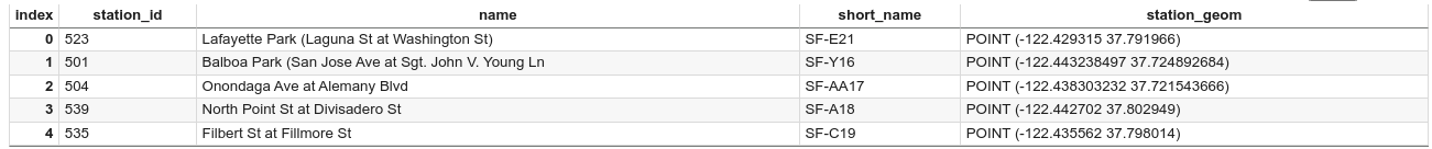
コードセルを挿入するには、[ コード] をクリックします。
station_geom列から経度と緯度の値を抽出するには、次のコードを入力します。# Extract the longitude (x) and latitude (y) from station_geom. gdf_sf_bikestations["longitude"] = gdf_sf_bikestations["station_geom"].x gdf_sf_bikestations["latitude"] = gdf_sf_bikestations["station_geom"].y
[ Run cell] をクリックします。
コードを実行しても、Colab ノートブックに出力は生成されません。セルの横にあるチェックマークは、コードが正常に実行されたことを示します。
コードセルを挿入するには、[ コード] をクリックします。
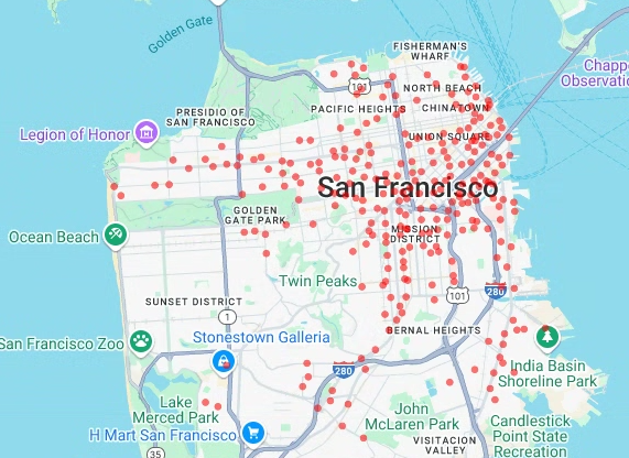
前に抽出した経度と緯度の値に基づいてシェアサイクル ステーションの散布図をレンダリングするには、次のコードを入力します。
# Render a scatter plot using pydeck with the extracted longitude and
# latitude columns in the gdf_sf_bikestations geopandas.GeoDataFrame.
scatterplot_layer = pdk.Layer(
  "ScatterplotLayer",
  id="bike_stations_scatterplot",
  data=gdf_sf_bikestations,
  get_position=['longitude', 'latitude'],
  get_radius=100,
  get_fill_color=[255, 0, 0, 140],  # Adjust color as desired
  pickable=True,
)

view_state = pdk.ViewState(latitude=37.77613, longitude=-122.42284, zoom=12)
display_pydeck_map([scatterplot_layer], view_state)
[ Run cell] をクリックします。
出力は次のようになります。
- 点
- 線
- ポリゴン
- マルチポリゴン
コードセルを挿入するには、[ コード] をクリックします。
サンフランシスコのエリア データセットの
bigquery-public-data.san_francisco_neighborhoods.boundariesテーブルから地理データをクエリするには、次のコードを入力します。このコードでは、%%bigqueryマジック関数を使用してクエリを実行し、結果を DataFrame で返します。# Query the neighborhood name and geometry from the San Francisco # neighborhoods dataset. %%bigquery gdf_sanfrancisco_neighborhoods --project {GCP_PROJECT_ID} --use_geodataframe geometry SELECT neighborhood, neighborhood_geom AS geometry FROM `bigquery-public-data.san_francisco_neighborhoods.boundaries`
[ Run cell] をクリックします。
出力は次のようになります。
Job ID 12345-1234-5678-1234-123456789 successfully executed: 100%コードセルを挿入するには、[ コード] をクリックします。
DataFrame の概要を取得するには、次のコードを入力します。
# Get a summary of the DataFrame
gdf_sanfrancisco_neighborhoods.info()
[ Run cell] をクリックします。
結果は次のようになります。
<class 'geopandas.geodataframe.GeoDataFrame'>
RangeIndex: 117 entries, 0 to 116
Data columns (total 2 columns):
#   Column        Non-Null Count  Dtype
---  ------        --------------  -----
0   neighborhood  117 non-null    object
1   geometry      117 non-null    geometry
dtypes: geometry(1), object(1)
memory usage: 2.0+ KB
DataFrame の最初の行をプレビューするには、次のコードを入力します。
# Preview the first row
gdf_sanfrancisco_neighborhoods.head(1)
[ Run cell] をクリックします。
出力は次のようになります。
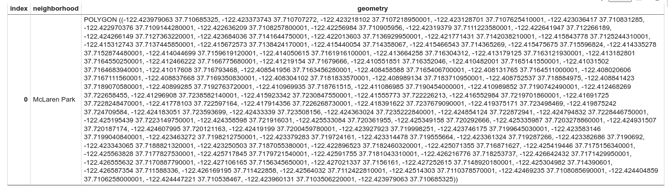
結果のデータはポリゴンであることに注意してください。
コードセルを挿入するには、[ コード] をクリックします。
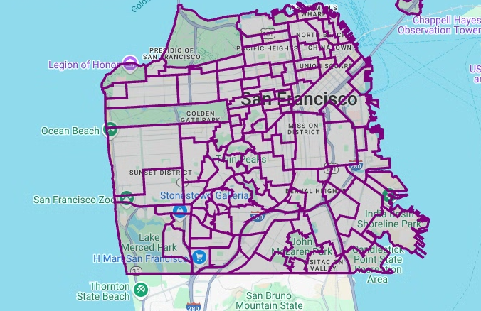
ポリゴンを可視化するには、次のコードを入力します。
pydeckは、ジオメトリ列内の各shapelyオブジェクト インスタンスをGeoJSON形式に変換するために使用されます。# Visualize the polygons. geojson_layer = pdk.Layer( 'GeoJsonLayer', id="sf_neighborhoods", data=gdf_sanfrancisco_neighborhoods, get_line_color=[127, 0, 127, 255], get_fill_color=[60, 60, 60, 50], get_line_width=100, pickable=True, stroked=True, filled=True, ) view_state = pdk.ViewState(latitude=37.77613, longitude=-122.42284, zoom=12) display_pydeck_map([geojson_layer], view_state)
[ Run cell] をクリックします。
出力は次のようになります。
コードセルを挿入するには、[ コード] をクリックします。
エリアごとのステーションの数を集計してカウントし、点の配列を含む
polygon列を作成するには、次のコードを入力します。# Aggregate and count the number of stations per neighborhood. gdf_count_stations = gdf_sanfrancisco_neighborhoods.sjoin(gdf_sf_bikestations, how='left', predicate='contains') gdf_count_stations = gdf_count_stations.groupby(by='neighborhood')['station_id'].count().rename('num_stations') gdf_stations_x_neighborhood = gdf_sanfrancisco_neighborhoods.join(gdf_count_stations, on='neighborhood', how='inner') # To simulate non-GeoJSON input data, create a polygon column that contains # an array of points by using the pandas.Series.map method. gdf_stations_x_neighborhood['polygon'] = gdf_stations_x_neighborhood['geometry'].map(lambda g: list(g.exterior.coords))
[ Run cell] をクリックします。
コードを実行しても、Colab ノートブックに出力は生成されません。セルの横にあるチェックマークは、コードが正常に実行されたことを示します。
コードセルを挿入するには、[ コード] をクリックします。
各ポリゴンに
fill_color列を追加するには、次のコードを入力します。# Create a color map gradient using the branch library, and add a fill_color # column for each of the polygons. colormap = branca.colormap.LinearColormap( colors=["lightblue", "darkred"], vmin=0, vmax=gdf_stations_x_neighborhood['num_stations'].max(), ) gdf_stations_x_neighborhood['fill_color'] = gdf_stations_x_neighborhood['num_stations'] \ .map(lambda c: list(colormap.rgba_bytes_tuple(c)[:3]) + [0.7 * 255]) # force opacity of 0.7
[ Run cell] をクリックします。
コードを実行しても、Colab ノートブックに出力は生成されません。セルの横にあるチェックマークは、コードが正常に実行されたことを示します。
コードセルを挿入するには、[ コード] をクリックします。
ポリゴンレイヤをレンダリングするには、次のコードを入力します。
# Render the polygon layer.
polygon_layer = pdk.Layer(
  'PolygonLayer',
  id="bike_stations_choropleth",
  data=gdf_stations_x_neighborhood,
  get_polygon='polygon',
  get_fill_color='fill_color',
  get_line_color=[0, 0, 0, 255],
  get_line_width=50,
  pickable=True,
  stroked=True,
  filled=True,
)
view_state = pdk.ViewState(latitude=37.77613, longitude=-122.42284, zoom=12)
display_pydeck_map([polygon_layer], view_state)
[ Run cell] をクリックします。
出力は次のようになります。
コードセルを挿入するには、[ コード] をクリックします。
サンフランシスコ警察署(SFPD)の報告データセットのデータをクエリするには、次のコードを入力します。このコードでは、
%%bigqueryマジック関数を使用してクエリを実行し、結果を DataFrame で返します。# Query the incident key and location data from the SFPD reports dataset. %%bigquery gdf_incidents --project {GCP_PROJECT_ID} --use_geodataframe location_geography SELECT unique_key, location_geography FROM ( SELECT unique_key, SAFE.ST_GEOGFROMTEXT(location) AS location_geography, # WKT string to GEOMETRY EXTRACT(YEAR FROM timestamp) AS year, FROM `bigquery-public-data.san_francisco_sfpd_incidents.sfpd_incidents` incidents ) WHERE year = 2015
[ Run cell] をクリックします。
出力は次のようになります。
Job ID 12345-1234-5678-1234-123456789 successfully executed: 100%コードセルを挿入するには、[ コード] をクリックします。
各インシデントの緯度と経度のセルを計算し、各セルのインシデントを集計して
geopandasDataFrame を作成し、ヒートマップ レイヤの各六角形の中心を追加するには、次のコードを入力します。# Compute the cell for each incident's latitude and longitude. H3_RESOLUTION = 9 gdf_incidents['h3_cell'] = gdf_incidents.geometry.apply( lambda geom: h3.latlng_to_cell(geom.y, geom.x, H3_RESOLUTION) ) # Aggregate the incidents for each hexagon cell. count_incidents = gdf_incidents.groupby(by='h3_cell')['unique_key'].count().rename('num_incidents') # Construct a new geopandas.GeoDataFrame with the aggregate results. # Add the center of each hexagon for the HeatmapLayer to render. gdf_incidents_x_cell = gpd.GeoDataFrame(data=count_incidents).reset_index() gdf_incidents_x_cell['h3_center'] = gdf_incidents_x_cell['h3_cell'].apply(h3.cell_to_latlng) gdf_incidents_x_cell.info()
[ Run cell] をクリックします。
出力は次のようになります。
<class 'geopandas.geodataframe.GeoDataFrame'>
RangeIndex: 969 entries, 0 to 968
Data columns (total 3 columns):
#   Column         Non-Null Count  Dtype
--  ------         --------------  -----
0   h3_cell        969 non-null    object
1   num_incidents  969 non-null    Int64
2   h3_center      969 non-null    object
dtypes: Int64(1), object(2)
memory usage: 23.8+ KB
コードセルを挿入するには、[ コード] をクリックします。
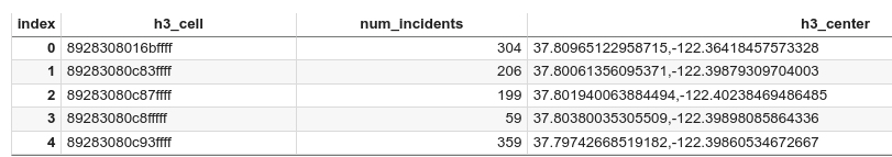
DataFrame の最初の 5 行をプレビューするには、次のコードを入力します。
# Preview the first five rows.
gdf_incidents_x_cell.head()
[ Run cell] をクリックします。
出力は次のようになります。
コードセルを挿入するには、[ コード] をクリックします。
データを
HeatmapLayerで使用できる JSON 形式に変換するには、次のコードを入力します。# Convert to a JSON format recognized by the HeatmapLayer. def _make_heatmap_datum(row) -> dict: return { "latitude": row['h3_center'][0], "longitude": row['h3_center'][1], "weight": float(row['num_incidents']), } heatmap_data = gdf_incidents_x_cell.apply(_make_heatmap_datum, axis='columns').values.tolist()
[ Run cell] をクリックします。
コードを実行しても、Colab ノートブックに出力は生成されません。セルの横にあるチェックマークは、コードが正常に実行されたことを示します。
コードセルを挿入するには、[ コード] をクリックします。
ヒートマップをレンダリングするには、次のコードを入力します。
# Render the heatmap.
heatmap_layer = pdk.Layer(
  "HeatmapLayer",
  id="sfpd_heatmap",
  data=heatmap_data,
  get_position=['longitude', 'latitude'],
  get_weight='weight',
  opacity=0.7,
  radius_pixels=99,  # this limitation can introduce artifacts (see above)
  aggregation='MEAN',
)
view_state = pdk.ViewState(latitude=37.77613, longitude=-122.42284, zoom=12)
display_pydeck_map([heatmap_layer], view_state)
[ Run cell] をクリックします。
出力は次のようになります。
- In the Google Cloud console, go to the Manage resources page.
- In the project list, select the project that you want to delete, and then click Delete.
- In the dialog, type the project ID, and then click Shut down to delete the project.
- In the Google Cloud console, go to the Manage resources page.
- In the project list, select the project that you want to delete, and then click Delete.
- In the dialog, type the project ID, and then click Shut down to delete the project.
Colab で、[ Secrets] をクリックします。
GMP_API_KEY行の末尾にある [Delete] をクリックします。省略可: ノートブックを削除するには、[ファイル] > [ゴミ箱に移動] をクリックします。
- BigQuery の地理空間分析の詳細については、BigQuery の地理空間分析の概要をご覧ください。
- BigQuery で地理空間データを可視化する方法については、地理空間データを可視化するをご覧ください。
pydeckや他のdeck.glグラフの種類について詳しくは、pydeckギャラリー、deck.glレイヤカタログ、deck.glGitHub ソースでサンプルをご覧ください。- データフレームでの地理空間データの操作の詳細については、GeoPandas のスタートガイド ページと GeoPandas ユーザーガイドをご覧ください。
- 幾何学的オブジェクトの操作の詳細については、Shapely ユーザー マニュアルをご覧ください。
- BigQuery で Google Earth Engine データを使用する方法については、Google Earth Engine のドキュメントの BigQuery へのエクスポートをご覧ください。
必要なロール
新しいプロジェクトを作成する場合、作成者がそのプロジェクトのオーナーとなり、このチュートリアルを完了するために必要なすべての IAM 権限が付与されます。
既存のプロジェクトを使用している場合、クエリジョブを実行するには、次のプロジェクト レベルのロールが必要です。
Make sure that you have the following role or roles on the project:
Check for the roles
Grant the roles
BigQuery のロールの詳細については、事前定義された IAM ロールをご覧ください。
Colab ノートブックを作成する
このチュートリアルでは、Colab ノートブックを作成して地理空間分析データを可視化します。Colab、Colab Enterprise、BigQuery Studio でノートブックのビルド済みバージョンを開くには、GitHub バージョンのチュートリアル(Colab での BigQuery 地理空間の可視化)の上部にあるリンクをクリックします。
Google Cloud と Google マップによる認証
このチュートリアルでは、BigQuery データセットに対してクエリを実行し、Google Maps JavaScript API を使用します。これらのリソースを使用するには、 Google Cloud と Maps API を使用して Colab ランタイムを認証します。
Google Cloudによる認証
省略可: Google マップで認証する
基本地図の地図プロバイダとして Google Maps Platform を使用する場合は、Google Maps Platform API キーを指定する必要があります。ノートブックは、Colab Secrets からキーを取得します。
この手順は、Maps API を使用している場合にのみ必要です。Google Maps Platform で認証しない場合、pydeck は代わりに carto マップを使用します。
Python パッケージをインストールしてデータ サイエンス ライブラリをインポートする
このチュートリアルでは、colabtools (google.colab)Python モジュールに加えて、他のいくつかの Python パッケージとデータ サイエンス ライブラリを使用します。
このセクションでは、pydeck パッケージと h3 パッケージをインストールします。pydeck は、deck.gl を活用した Python での大規模な空間レンダリングを提供します。h3-py は、Uber の H3 Hexagonal Hierarchical Geospatial Indexing System を Python で提供します。
次に、h3 ライブラリと pydeck ライブラリと、次の Python 地理空間ライブラリをインポートします。
ライブラリをインポートしたら、Colab の pandas DataFrame でインタラクティブなテーブルを有効にします。
pydeck パッケージと h3 パッケージをインストールします
Python ライブラリをインポートする
pandas DataFrame のインタラクティブなテーブルを有効にする
共有ルーティンを作成する
このセクションでは、基本地図上にレイヤをレンダリングする共有ルーティンを作成します。
散布図を作成する
このセクションでは、bigquery-public-data.san_francisco_bikeshare.bikeshare_station_info テーブルからデータを取得して、サンフランシスコの Ford GoBike Share 一般公開データセット内のすべてのシェアサイクル ステーションの散布図を作成します。散布図は、deck.gl フレームワークのレイヤと散布図レイヤを使用して作成されます。
散布図は、個々の点のサブセットを確認する(スポット チェックとも呼ばれます)必要がある場合に便利です。
次の例は、レイヤと散布図レイヤを使用して個々の点を円としてレンダリングする方法を示しています。
点をレンダリングするには、シェアサイクル データセットの station_geom 列から経度と緯度を x 座標と y 座標として抽出する必要があります。
gdf_sf_bikestations は geopandas.GeoDataFrame であるため、座標は station_geom ジオメトリ列から直接アクセスされます。経度は列の .x 属性、緯度は列の .y 属性を使用して取得できます。その後、取得した値をそれぞれ新しい経度と緯度の列に格納できます。
ポリゴンを可視化する
地理空間分析では、GEOGRAPHY データ型と標準の GoogleSQL 地理関数を使用して、BigQuery で地理空間データを分析し、可視化できます。
地理空間分析での GEOGRAPHY データ型は、点、LineString、ポリゴンのコレクションであり、点セットまたは地球表面のサブセットとして表されます。GEOGRAPHY 型には、次のようなオブジェクトを含めることができます。
サポートされているすべてのオブジェクトの一覧については、GEOGRAPHY 型のドキュメントをご覧ください。
想定されるシェイプがわからない地理空間データが提供されている場合は、データを可視化してシェイプを検出できます。地理データを GeoJSON 形式に変換すると、シェイプを可視化できます。deck.gl フレームワークの GeoJSON レイヤを使用して、GeoJSON データを可視化できます。
このセクションでは、サンフランシスコのエリア データセットの地理データをクエリし、ポリゴンを可視化します。
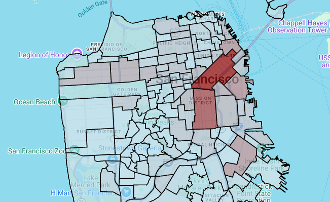
階級区分図を作成する
GeoJSON 形式に変換するのが困難なポリゴンを含むデータを探索する場合は、代わりに deck.gl フレームワークのポリゴンレイヤを使用できます。ポリゴンレイヤは、点の配列など、特定のタイプの入力データを処理できます。
このセクションでは、ポリゴンレイヤを使用して点の配列をレンダリングし、その結果を使用して階級区分図をレンダリングします。階級区分図は、サンフランシスコのエリア データセットとサンフランシスコの Ford GoBike Share データセットのデータを結合して、シェアサイクル ステーションの密度をエリア別に示しています。
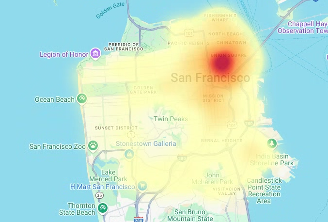
ヒートマップを作成する
階級区分は、既知の意味のある境界がある場合に便利です。既知の意味のある境界がないデータがある場合は、ヒートマップ レイヤを使用して連続的な密度をレンダリングできます。
次の例では、サンフランシスコ警察署(SFPD)の報告データセットの bigquery-public-data.san_francisco_sfpd_incidents.sfpd_incidents テーブルのデータをクエリします。このデータは、2015 年のインシデントの分布を可視化するために使用されます。
ヒートマップの場合は、レンダリングする前にデータを量子化して集計することをおすすめします。この例では、Carto の H3 空間インデックスを使用してデータが量子化され、集計されます。ヒートマップは、deck.gl フレームワークのヒートマップ レイヤを使用して作成されます。
この例では、h3 Python ライブラリを使用して量子化を行い、インシデントのを六角形に集約します。h3.latlng_to_cell 関数は、インシデントの位置(緯度と経度)を H3 セル インデックスにマッピングするために使用されます。H3 解像度を 9 にすると、ヒートマップ用の十分に集約された六角形が得られます。h3.cell_to_latlng 関数は、各六角形の中心を決定するために使用されます。
クリーンアップ
このチュートリアルで使用したリソースについて、Google Cloud アカウントに課金されないようにするには、リソースを含むプロジェクトを削除するか、プロジェクトを維持して個々のリソースを削除します。
プロジェクトの削除
コンソール
gcloud
Google Maps API キーとノートブックを削除する
Google Cloud プロジェクトを削除した後、Google Maps API を使用した場合は、Colab Secrets から Google Maps API キーを削除し、必要に応じてノートブックを削除します。