在本教程中,您将使用 Colab 笔记本直观呈现 BigQuery 中的地理空间分析数据。
本教程使用以下 BigQuery 公共数据集:
如需了解如何访问这些公共数据集,请参阅在 Google Cloud 控制台中访问公共数据集。
您可以使用公共数据集创建以下可视化图表:
- Ford GoBike 共享数据集中所有共享单车站的散点图
- 旧金山街区数据集中的多边形
- 按街区显示共享单车站数量的分级统计图
- 旧金山警察局 (SFPD) 报告数据集中的突发事件热图
目标
- 使用 Google Cloud 设置身份验证,并视情况添加 Google 地图。
- 在 BigQuery 中查询数据,并将结果下载到 Colab 中。
- 使用 Python 数据科学工具执行转换和分析。
- 创建可视化图表,包括散点图、多边形、分级统计图和热图。
费用
在本文档中,您将使用 Google Cloud的以下收费组件:
如需根据您的预计使用量来估算费用,请使用价格计算器。
完成本文档中描述的任务后,您可以通过删除所创建的资源来避免继续计费。如需了解详情,请参阅清理。
准备工作
- Sign in to your Google Cloud account. If you're new to Google Cloud, create an account to evaluate how our products perform in real-world scenarios. New customers also get $300 in free credits to run, test, and deploy workloads.
-
In the Google Cloud console, on the project selector page, select or create a Google Cloud project.
Roles required to select or create a project
- Select a project: Selecting a project doesn't require a specific IAM role—you can select any project that you've been granted a role on.
-
Create a project: To create a project, you need the Project Creator
(
roles/resourcemanager.projectCreator), which contains theresourcemanager.projects.createpermission. Learn how to grant roles.
-
Verify that billing is enabled for your Google Cloud project.
-
Enable the BigQuery and Google Maps JavaScript APIs.
Roles required to enable APIs
To enable APIs, you need the Service Usage Admin IAM role (
roles/serviceusage.serviceUsageAdmin), which contains theserviceusage.services.enablepermission. Learn how to grant roles. -
In the Google Cloud console, on the project selector page, select or create a Google Cloud project.
Roles required to select or create a project
- Select a project: Selecting a project doesn't require a specific IAM role—you can select any project that you've been granted a role on.
-
Create a project: To create a project, you need the Project Creator
(
roles/resourcemanager.projectCreator), which contains theresourcemanager.projects.createpermission. Learn how to grant roles.
-
Verify that billing is enabled for your Google Cloud project.
-
Enable the BigQuery and Google Maps JavaScript APIs.
Roles required to enable APIs
To enable APIs, you need the Service Usage Admin IAM role (
roles/serviceusage.serviceUsageAdmin), which contains theserviceusage.services.enablepermission. Learn how to grant roles. - 确保您拥有必要的权限,以便执行本文档中的任务。
- BigQuery User (
roles/bigquery.user) -
In the Google Cloud console, go to the IAM page.
Go to IAM - Select the project.
-
In the Principal column, find all rows that identify you or a group that you're included in. To learn which groups you're included in, contact your administrator.
- For all rows that specify or include you, check the Role column to see whether the list of roles includes the required roles.
-
In the Google Cloud console, go to the IAM page.
前往 IAM - 选择项目。
- 点击 授予访问权限。
-
在新的主账号字段中,输入您的用户标识符。 这通常是 Google 账号的电子邮件地址。
- 在选择角色列表中,选择一个角色。
- 如需授予其他角色,请点击 添加其他角色,然后添加其他各个角色。
- 点击 Save(保存)。
打开 Colab。
在打开笔记本对话框中,点击新建笔记本。
点击
Untitled0.ipynb,然后将笔记本的名称更改为bigquery-geo.ipynb。选择文件 > 保存。
如需插入代码单元,请点击 代码。
如需使用项目进行身份验证,请输入以下代码:
# REQUIRED: Authenticate with your project.
GCP_PROJECT_ID = "PROJECT_ID"  #@param {type:"string"}

from google.colab import auth
from google.colab import userdata

auth.authenticate_user(project_id=GCP_PROJECT_ID)

# Set GMP_API_KEY to none
GMP_API_KEY = None
将 PROJECT_ID 替换为您的项目 ID。
点击 运行单元。
出现提示时,如果您同意,请点击允许,以授予 Colab 访问您的凭证的权限。
在使用 Google 账号登录页面上,选择您的账号。
在登录第三方创建的笔记本代码页面上,点击继续。
在选择第三方创建的笔记本代码可以访问的内容页面上,点击全选,然后点击继续。
完成授权流程后,Colab 笔记本中不会生成任何输出。单元格旁边的对勾标记表示代码已成功运行。
按照 Google 地图文档中使用 API 密钥页面上的说明,获取 Google 地图 API 密钥。
切换到您的 Colab 笔记本,然后点击 Secret。
点击添加新 Secret。
对于名称,请输入
GMP_API_KEY。在值字段中,输入您之前生成的 Maps API 密钥值。
关闭 Secret 面板。
如需插入代码单元,请点击 代码。
如需使用 Maps API 进行身份验证,请输入以下代码:
# Authenticate with the Google Maps JavaScript API.
GMP_API_SECRET_KEY_NAME = "GMP_API_KEY" #@param {type:"string"}

if GMP_API_SECRET_KEY_NAME:
  GMP_API_KEY = userdata.get(GMP_API_SECRET_KEY_NAME) if GMP_API_SECRET_KEY_NAME else None
else:
  GMP_API_KEY = None
出现提示时,如果您同意,点击授予访问权限,以授予笔记本访问您的密钥的权限。
点击 运行单元。
完成授权流程后,Colab 笔记本中不会生成任何输出。单元格旁边的对勾标记表示代码已成功运行。
geopandas,用于扩展pandas所用的数据类型,以允许对几何类型执行空间操作。shapely,用于操控和分析各个平面几何对象。branca,用于生成 HTML 和 JavaScript 色图。geemap.deck,用于使用pydeck和earthengine-api进行可视化。如需插入代码单元,请点击 代码。
如需安装
pydeck和h3软件包,请输入以下代码:# Install pydeck and h3. !pip install pydeck>=0.9 h3>=4.2
点击 运行单元。
完成安装后,Colab 笔记本中不会生成任何输出。单元格旁边的对勾标记表示代码已成功运行。
如需插入代码单元,请点击 代码。
如需导入 Python 库,请输入以下代码:
# Import data science libraries.
import branca
import geemap.deck as gmdk
import h3
import pydeck as pdk
import geopandas as gpd
import shapely
点击 运行单元。
运行代码后,Colab 笔记本中不会生成任何输出。单元格旁边的对勾标记表示代码已成功运行。
如需插入代码单元,请点击 代码。
如需启用
pandasDataFrames,请输入以下代码:# Enable displaying pandas data frames as interactive tables by default. from google.colab import data_table data_table.enable_dataframe_formatter()
点击 运行单元。
运行代码后,Colab 笔记本中不会生成任何输出。单元格旁边的对勾标记表示代码已成功运行。
如需插入代码单元,请点击 代码。
如需创建用于在地图上渲染图层的共享例程,请输入以下代码:
# Set Google Maps as the base map provider.
MAP_PROVIDER_GOOGLE = pdk.bindings.base_map_provider.BaseMapProvider.GOOGLE_MAPS.value

# Shared routine for rendering layers on a map using geemap.deck.
def display_pydeck_map(layers, view_state, **kwargs):
  deck_kwargs = kwargs.copy()

  # Use Google Maps as the base map only if the API key is provided.
  if GMP_API_KEY:
    deck_kwargs.update({
      "map_provider": MAP_PROVIDER_GOOGLE,
      "map_style": pdk.bindings.map_styles.GOOGLE_ROAD,
      "api_keys": {MAP_PROVIDER_GOOGLE: GMP_API_KEY},
    })

  m = gmdk.Map(initial_view_state=view_state, ee_initialize=False, **deck_kwargs)

  for layer in layers:
    m.add_layer(layer)
  return m
点击 运行单元。
运行代码后,Colab 笔记本中不会生成任何输出。单元格旁边的对勾标记表示代码已成功运行。
如需插入代码单元,请点击 代码。
如需查询旧金山福特 GoBike 共享单车公共数据集,请输入以下代码。此代码使用
%%bigquery魔术函数运行查询,并以 DataFrame 的形式返回结果:# Query the station ID, station name, station short name, and station # geometry from the bike share dataset. # NOTE: In this tutorial, the denormalized 'lat' and 'lon' columns are # ignored. They are decomposed components of the geometry. %%bigquery gdf_sf_bikestations --project {GCP_PROJECT_ID} --use_geodataframe station_geom SELECT station_id, name, short_name, station_geom FROM `bigquery-public-data.san_francisco_bikeshare.bikeshare_station_info`
点击 运行单元。
输出类似于以下内容:
Job ID 12345-1234-5678-1234-123456789 successfully executed: 100%如需插入代码单元,请点击 代码。
如需获取 DataFrame 的摘要(包括列和数据类型),请输入以下代码:
# Get a summary of the DataFrame
gdf_sf_bikestations.info()
点击 运行单元。
输出应如下所示:
<class 'geopandas.geodataframe.GeoDataFrame'>
RangeIndex: 472 entries, 0 to 471
Data columns (total 4 columns):
#   Column        Non-Null Count  Dtype
---  ------        --------------  -----
0   station_id    472 non-null    object
1   name          472 non-null    object
2   short_name    472 non-null    object
3   station_geom  472 non-null    geometry
dtypes: geometry(1), object(3)
memory usage: 14.9+ KB
如需插入代码单元,请点击 代码。
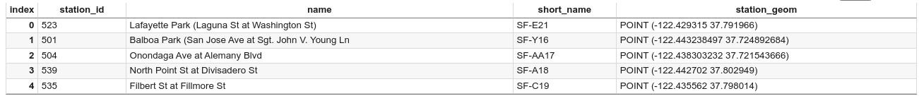
如需预览 DataFrame 的前五行,请输入以下代码:
# Preview the first five rows
gdf_sf_bikestations.head()
点击 运行单元。
输出类似于以下内容:
如需插入代码单元,请点击 代码。
如需从
station_geom列提取经度和纬度值,请输入以下代码:# Extract the longitude (x) and latitude (y) from station_geom. gdf_sf_bikestations["longitude"] = gdf_sf_bikestations["station_geom"].x gdf_sf_bikestations["latitude"] = gdf_sf_bikestations["station_geom"].y
点击 运行单元。
运行代码后,Colab 笔记本中不会生成任何输出。单元格旁边的对勾标记表示代码已成功运行。
如需插入代码单元,请点击 代码。
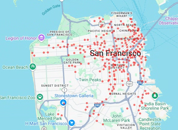
如需根据您之前提取的经纬度值渲染共享单车站点的散点图,请输入以下代码:
# Render a scatter plot using pydeck with the extracted longitude and
# latitude columns in the gdf_sf_bikestations geopandas.GeoDataFrame.
scatterplot_layer = pdk.Layer(
  "ScatterplotLayer",
  id="bike_stations_scatterplot",
  data=gdf_sf_bikestations,
  get_position=['longitude', 'latitude'],
  get_radius=100,
  get_fill_color=[255, 0, 0, 140],  # Adjust color as desired
  pickable=True,
)

view_state = pdk.ViewState(latitude=37.77613, longitude=-122.42284, zoom=12)
display_pydeck_map([scatterplot_layer], view_state)
点击 运行单元。
输出类似于以下内容:
- 积分
- 线条
- 多边形
- 多多边形
如需插入代码单元,请点击 代码。
如需查询旧金山街区数据集中
bigquery-public-data.san_francisco_neighborhoods.boundaries表中的地理数据,请输入以下代码。此代码使用%%bigquery魔术函数运行查询,并以 DataFrame 的形式返回结果:# Query the neighborhood name and geometry from the San Francisco # neighborhoods dataset. %%bigquery gdf_sanfrancisco_neighborhoods --project {GCP_PROJECT_ID} --use_geodataframe geometry SELECT neighborhood, neighborhood_geom AS geometry FROM `bigquery-public-data.san_francisco_neighborhoods.boundaries`
点击 运行单元。
输出类似于以下内容:
Job ID 12345-1234-5678-1234-123456789 successfully executed: 100%如需插入代码单元,请点击 代码。
如需获取 DataFrame 的摘要,请输入以下代码:
# Get a summary of the DataFrame
gdf_sanfrancisco_neighborhoods.info()
点击 运行单元。
结果应如下所示:
<class 'geopandas.geodataframe.GeoDataFrame'>
RangeIndex: 117 entries, 0 to 116
Data columns (total 2 columns):
#   Column        Non-Null Count  Dtype
---  ------        --------------  -----
0   neighborhood  117 non-null    object
1   geometry      117 non-null    geometry
dtypes: geometry(1), object(1)
memory usage: 2.0+ KB
如需预览 DataFrame 的第一行,请输入以下代码:
# Preview the first row
gdf_sanfrancisco_neighborhoods.head(1)
点击 运行单元。
输出类似于以下内容:
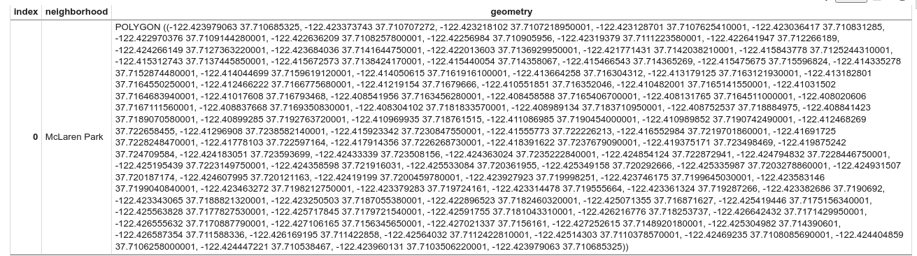
在结果中,请注意数据采用多边形格式。
如需插入代码单元,请点击 代码。
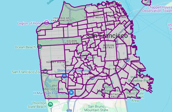
如需直观呈现多边形,请输入以下代码。
pydeck用于将几何图形列中的每个shapely对象实例转换为GeoJSON格式:# Visualize the polygons. geojson_layer = pdk.Layer( 'GeoJsonLayer', id="sf_neighborhoods", data=gdf_sanfrancisco_neighborhoods, get_line_color=[127, 0, 127, 255], get_fill_color=[60, 60, 60, 50], get_line_width=100, pickable=True, stroked=True, filled=True, ) view_state = pdk.ViewState(latitude=37.77613, longitude=-122.42284, zoom=12) display_pydeck_map([geojson_layer], view_state)
点击 运行单元。
输出类似于以下内容:
如需插入代码单元,请点击 代码。
如需汇总和统计每个街区的站点数量,并创建一个包含点数组的
polygon列,请输入以下代码:# Aggregate and count the number of stations per neighborhood. gdf_count_stations = gdf_sanfrancisco_neighborhoods.sjoin(gdf_sf_bikestations, how='left', predicate='contains') gdf_count_stations = gdf_count_stations.groupby(by='neighborhood')['station_id'].count().rename('num_stations') gdf_stations_x_neighborhood = gdf_sanfrancisco_neighborhoods.join(gdf_count_stations, on='neighborhood', how='inner') # To simulate non-GeoJSON input data, create a polygon column that contains # an array of points by using the pandas.Series.map method. gdf_stations_x_neighborhood['polygon'] = gdf_stations_x_neighborhood['geometry'].map(lambda g: list(g.exterior.coords))
点击 运行单元。
运行代码后,Colab 笔记本中不会生成任何输出。单元格旁边的对勾标记表示代码已成功运行。
如需插入代码单元,请点击 代码。
如需为每个多边形添加
fill_color列,请输入以下代码:# Create a color map gradient using the branch library, and add a fill_color # column for each of the polygons. colormap = branca.colormap.LinearColormap( colors=["lightblue", "darkred"], vmin=0, vmax=gdf_stations_x_neighborhood['num_stations'].max(), ) gdf_stations_x_neighborhood['fill_color'] = gdf_stations_x_neighborhood['num_stations'] \ .map(lambda c: list(colormap.rgba_bytes_tuple(c)[:3]) + [0.7 * 255]) # force opacity of 0.7
点击 运行单元。
运行代码后,Colab 笔记本中不会生成任何输出。单元格旁边的对勾标记表示代码已成功运行。
如需插入代码单元,请点击 代码。
如需渲染多边形图层,请输入以下代码:
# Render the polygon layer.
polygon_layer = pdk.Layer(
  'PolygonLayer',
  id="bike_stations_choropleth",
  data=gdf_stations_x_neighborhood,
  get_polygon='polygon',
  get_fill_color='fill_color',
  get_line_color=[0, 0, 0, 255],
  get_line_width=50,
  pickable=True,
  stroked=True,
  filled=True,
)
view_state = pdk.ViewState(latitude=37.77613, longitude=-122.42284, zoom=12)
display_pydeck_map([polygon_layer], view_state)
点击 运行单元。
输出类似于以下内容:
如需插入代码单元,请点击 代码。
如需查询“旧金山警察局 (SFPD) 报告”数据集中的数据,请输入以下代码。此代码使用
%%bigquery魔术函数运行查询,并以 DataFrame 的形式返回结果:# Query the incident key and location data from the SFPD reports dataset. %%bigquery gdf_incidents --project {GCP_PROJECT_ID} --use_geodataframe location_geography SELECT unique_key, location_geography FROM ( SELECT unique_key, SAFE.ST_GEOGFROMTEXT(location) AS location_geography, # WKT string to GEOMETRY EXTRACT(YEAR FROM timestamp) AS year, FROM `bigquery-public-data.san_francisco_sfpd_incidents.sfpd_incidents` incidents ) WHERE year = 2015
点击 运行单元。
输出类似于以下内容:
Job ID 12345-1234-5678-1234-123456789 successfully executed: 100%如需插入代码单元,请点击 代码。
如需计算每个突发事件的纬度和经度对应的单元格、汇总每个单元格的突发事件、构建
geopandasDataFrame,并为热图图层添加每个六边形的中心点,请输入以下代码:# Compute the cell for each incident's latitude and longitude. H3_RESOLUTION = 9 gdf_incidents['h3_cell'] = gdf_incidents.geometry.apply( lambda geom: h3.latlng_to_cell(geom.y, geom.x, H3_RESOLUTION) ) # Aggregate the incidents for each hexagon cell. count_incidents = gdf_incidents.groupby(by='h3_cell')['unique_key'].count().rename('num_incidents') # Construct a new geopandas.GeoDataFrame with the aggregate results. # Add the center of each hexagon for the HeatmapLayer to render. gdf_incidents_x_cell = gpd.GeoDataFrame(data=count_incidents).reset_index() gdf_incidents_x_cell['h3_center'] = gdf_incidents_x_cell['h3_cell'].apply(h3.cell_to_latlng) gdf_incidents_x_cell.info()
点击 运行单元。
输出类似于以下内容:
<class 'geopandas.geodataframe.GeoDataFrame'>
RangeIndex: 969 entries, 0 to 968
Data columns (total 3 columns):
#   Column         Non-Null Count  Dtype
--  ------         --------------  -----
0   h3_cell        969 non-null    object
1   num_incidents  969 non-null    Int64
2   h3_center      969 non-null    object
dtypes: Int64(1), object(2)
memory usage: 23.8+ KB
如需插入代码单元,请点击 代码。
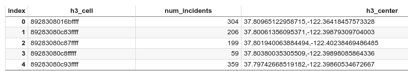
如需预览 DataFrame 的前五行,请输入以下代码:
# Preview the first five rows.
gdf_incidents_x_cell.head()
点击 运行单元。
输出类似于以下内容:
如需插入代码单元,请点击 代码。
如需将数据转换为可供
HeatmapLayer使用的 JSON 格式,请输入以下代码:# Convert to a JSON format recognized by the HeatmapLayer. def _make_heatmap_datum(row) -> dict: return { "latitude": row['h3_center'][0], "longitude": row['h3_center'][1], "weight": float(row['num_incidents']), } heatmap_data = gdf_incidents_x_cell.apply(_make_heatmap_datum, axis='columns').values.tolist()
点击 运行单元。
运行代码后,Colab 笔记本中不会生成任何输出。单元格旁边的对勾标记表示代码已成功运行。
如需插入代码单元,请点击 代码。
如需渲染热图,请输入以下代码:
# Render the heatmap.
heatmap_layer = pdk.Layer(
  "HeatmapLayer",
  id="sfpd_heatmap",
  data=heatmap_data,
  get_position=['longitude', 'latitude'],
  get_weight='weight',
  opacity=0.7,
  radius_pixels=99,  # this limitation can introduce artifacts (see above)
  aggregation='MEAN',
)
view_state = pdk.ViewState(latitude=37.77613, longitude=-122.42284, zoom=12)
display_pydeck_map([heatmap_layer], view_state)
点击 运行单元。
输出类似于以下内容:
- In the Google Cloud console, go to the Manage resources page.
- In the project list, select the project that you want to delete, and then click Delete.
- In the dialog, type the project ID, and then click Shut down to delete the project.
- In the Google Cloud console, go to the Manage resources page.
- In the project list, select the project that you want to delete, and then click Delete.
- In the dialog, type the project ID, and then click Shut down to delete the project.
在 Colab 中,点击 Secret。
在
GMP_API_KEY行末尾,点击 删除。(可选)如需删除笔记本,请点击文件 > 移至回收站。
- 如需详细了解 BigQuery 中的地理空间分析,请参阅 BigQuery 中地理空间分析简介。
- 如需了解如何在 BigQuery 中直观呈现地理空间数据,请参阅直观呈现地理空间数据。
- 如需详细了解
pydeck和其他deck.gl图表类型,您可以在pydeck图库、deck.gl图层目录和deck.glGitHub 源代码中找到示例。 - 如需详细了解如何在 DataFrame 中使用地理空间数据,请参阅 GeoPandas 入门页面和 GeoPandas 用户指南。
- 如需详细了解几何对象操纵,请参阅 Shapely 用户手册。
- 如需探索如何在 BigQuery 中使用 Google Earth Engine 数据,请参阅 Google Earth Engine 文档中的导出到 BigQuery。
所需的角色
如果您创建了一个新项目,那么您就是项目所有者,并且会获得完成本教程所需的所有必要 IAM 权限。
如果您要使用现有项目,则需要具备以下项目级角色才能运行查询作业。
Make sure that you have the following role or roles on the project:
Check for the roles
Grant the roles
如需详细了解 BigQuery 中的角色,请参阅预定义的 IAM 角色。
创建 Colab 笔记本
本教程将构建一个 Colab 笔记本,以直观呈现地理空间分析数据。您可以通过点击 GitHub 版教程顶部的链接,在 Colab、Colab Enterprise 或 BigQuery Studio 中打开笔记本的预构建版本 - Colab 中的 BigQuery 地理空间可视化。
使用 Google Cloud 和 Google 地图进行身份验证
本教程将查询 BigQuery 数据集并使用 Google Maps JavaScript API。如需使用这些资源,您可以使用 Google Cloud 和 Maps API 对 Colab 运行时进行身份验证。
使用 Google Cloud进行身份验证
(可选)使用 Google 地图进行身份验证
如果您将 Google Maps Platform 用作底图的地图提供方,则必须提供 Google Maps Platform API 密钥。该笔记本会从您的 Colab Secret 中检索此密钥。
仅当您使用的是 Maps API 时,才需要执行此步骤。如果您不使用 Google Maps Platform 进行身份验证,pydeck 会改用 carto 地图。
安装 Python 软件包并导入数据科学库
除了 colabtools (google.colab) Python 模块之外,本教程还使用了其他一些 Python 软件包和数据科学库。
在本部分中,您将安装 pydeck 和 h3 软件包。pydeck 使用 deck.gl 提供支持,可在 Python 中提供大规模空间渲染。h3-py 在 Python 中提供了 Uber 的 H3 六边形分层地理空间索引系统。
然后,导入 h3 和 pydeck 库以及以下 Python 地理空间库:
导入库后,您可以为 Colab 中的 pandas DataFrames 启用交互式表格。
安装 pydeck 和 h3 软件包。
导入 Python 库
为 pandas DataFrames 启用交互式表格
创建共享例程
在本部分中,您将创建一个在底图上渲染图层的共享例程。
创建散点图
在本部分中,您将通过从 bigquery-public-data.san_francisco_bikeshare.bikeshare_station_info 表中检索数据,为旧金山福特 GoBike 共享单车公共数据集中的所有共享单车站创建散点图。散点图是使用图层和 deck.gl 框架中的散点图层创建的。
当您需要检查部分单个数据点(也称为抽查)时,散点图非常有用。
以下示例演示了如何使用图层和散点图图层将各个点渲染为圆形。
要渲染这些点,您需要从共享单车数据集的 station_geom 列中提取经度和纬度,并将其作为 x 和 y 坐标。
由于 gdf_sf_bikestations 是一个 geopandas.GeoDataFrame,因此可以直接通过其 station_geom 几何图形列访问坐标。您可以使用该列的 .x 属性检索经度,并使用其 .y 属性检索纬度。然后,您可以将其存储在新的经度和纬度列中。
直观呈现多边形
借助地理空间分析,您可以使用 GEOGRAPHY 数据类型和 GoogleSQL 地理函数来分析和直观呈现 BigQuery 中的地理空间数据。
地理空间分析中的 GEOGRAPHY 数据类型是点、线串和多边形的集合,表示为一个点集或地球表面的子集。GEOGRAPHY 类型可以包含以下对象:
如需查看所有受支持对象的列表,请参阅 GEOGRAPHY 类型文档。
如果您不知道所提供的地理空间数据的预期形状,可以通过直观呈现数据来发现形状。您可以通过将地理数据转换为 GeoJSON 格式来直观呈现形状。然后,您可以使用 deck.gl 框架中的 GeoJSON 图层直观呈现 GeoJSON 数据。
在本部分中,您将查询旧金山街区数据集中的地理数据,然后直观呈现多边形。
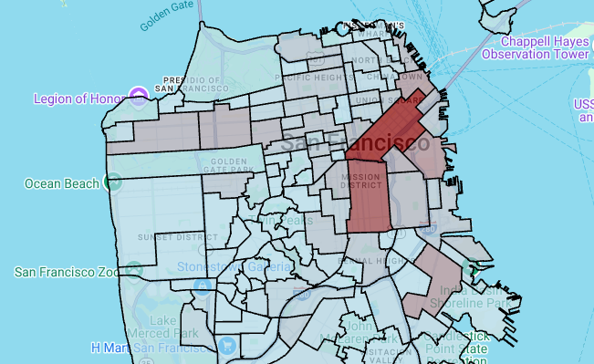
创建分级统计图
如果您要探索的数据包含难以转换为 GeoJSON 格式的多边形,则可以改用 deck.gl 框架中的多边形图层。多边形图层可以处理特定类型的输入数据,例如点的数组。
在本部分中,您将使用多边形图层来渲染点数组,并使用结果来渲染分级统计图。通过将旧金山街区数据集的数据与旧金山福特 GoBike 共享单车数据集的数据联接,此分级统计图显示了按街区划分的共享单车站点密度。
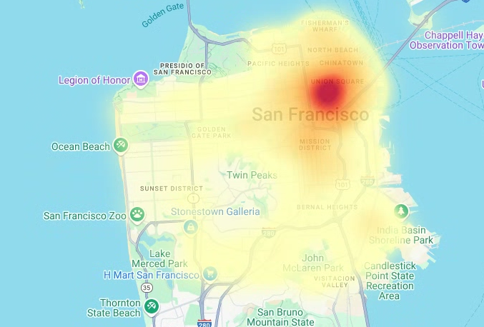
创建热图
当您拥有已知的、有意义的边界时,分级统计图非常有用。如果您的数据没有已知的、有意义的边界,则可以使用热图图层来渲染其连续密度。
在以下示例中,您将查询旧金山警察局 (SFPD) 报告数据集中的 bigquery-public-data.san_francisco_sfpd_incidents.sfpd_incidents 表中的数据。这些数据用于直观呈现 2015 年突发事件的分布情况。
对于热图,建议您在渲染之前对数据进行量化和汇总。在此示例中,数据使用 Carto H3 空间索引进行量化和汇总。热图是使用 deck.gl 框架中的热图图层创建的。
在此示例中,我们使用 h3 Python 库将事件点汇总到六边形中,以实现量化。h3.latlng_to_cell 函数用于将突发事件位置(纬度和经度)映射到 H3 单元格索引。H3 分辨率为 9 时,热图可获得足够的汇总六边形。h3.cell_to_latlng 函数用于确定每个六边形的中心。
清理
为避免因本教程中使用的资源导致您的 Google Cloud 账号产生费用,请删除包含这些资源的项目,或者保留项目但删除各个资源。
删除项目
控制台
gcloud
删除您的 Google 地图 API 密钥和笔记本
删除 Google Cloud 项目后,如果您使用了 Google 地图 API,请从 Colab Secrets 中删除 Google 地图 API 密钥,然后酌情删除笔记本。