从 JupyterLab 中探索和直观呈现 BigQuery 中的数据

本页面展示了一些示例，介绍如何从 Vertex AI Workbench 代管式笔记本实例的 JupyterLab 界面中探索和直观呈现存储在 BigQuery 中的数据。

准备工作

创建代管式笔记本实例（如果您尚未创建）。

打开 JupyterLab

在 Google Cloud 控制台中，前往代管式笔记本页面。

前往“代管式笔记本”
在代管式笔记本实例的名称旁边，点击打开 JupyterLab。

您的代管式笔记本实例会打开 JupyterLab。

从 BigQuery 中读取数据。

在接下来的两部分中，您将从 BigQuery 中读取数据以备后续直观呈现。这些步骤与从 JupyterLab 中查询 BigQuery 中的数据中的步骤相同，因此，如果您已完成这些步骤，则可以跳至获取 BigQuery 表中的数据摘要。

使用 %%bigquery 魔法命令查询数据

在本部分中，您可以直接在笔记本单元中写入 SQL，并将 BigQuery 中的数据读取到 Python 笔记本。

使用一个或两个百分比字符（% 或 %%）的魔法命令可让您使用最少的语法在笔记本中与 BigQuery 进行交互。Python 版 BigQuery 客户端库会自动安装在代管式笔记本实例中。在后台，%%bigquery 魔法命令使用 Python 版 BigQuery 客户端库运行给定查询，将结果转换为 Pandas DataFrame，以及视需要将结果保存到变量中，然后显示结果。

注意：从 google-cloud-bigquery Python 软件包 1.26.0 版开始，默认使用 BigQuery Storage API 从 %%bigquery 魔法命令下载结果。

如需打开笔记本文件，请选择文件 > 新建 > 笔记本。
在选择内核对话框中，选择 Python（本地），然后点击选择。

系统会打开您的新 IPYNB 文件。

如需获取 international_top_terms 数据集中国家/地区的区域数，请输入以下语句：

%%bigquery
SELECT
  country_code,
  country_name,
  COUNT(DISTINCT region_code) AS num_regions
FROM
  `bigquery-public-data.google_trends.international_top_terms`
WHERE
  refresh_date = DATE_SUB(CURRENT_DATE, INTERVAL 1 DAY)
GROUP BY
  country_code,
  country_name
ORDER BY
  num_regions DESC;

点击 运行单元。

输出类似于以下内容：

Query complete after 0.07s: 100%|██████████| 4/4 [00:00<00:00, 1440.60query/s]
Downloading: 100%|██████████| 41/41 [00:02<00:00, 20.21rows/s]
country_code      country_name    num_regions
0   TR  Turkey         81
1   TH  Thailand       77
2   VN  Vietnam        63
3   JP  Japan          47
4   RO  Romania        42
5   NG  Nigeria        37
6   IN  India          36
7   ID  Indonesia      34
8   CO  Colombia       33
9   MX  Mexico         32
10  BR  Brazil         27
11  EG  Egypt          27
12  UA  Ukraine        27
13  CH  Switzerland    26
14  AR  Argentina      24
15  FR  France         22
16  SE  Sweden         21
17  HU  Hungary        20
18  IT  Italy          20
19  PT  Portugal       20
20  NO  Norway         19
21  FI  Finland        18
22  NZ  New Zealand    17
23  PH  Philippines    17
...

在下一个单元（在上一个单元的输出下方）中，输入以下命令以运行相同查询，但这次会将结果保存到名为 regions_by_country 的新 Pandas DataFrame 中。您通过在 %%bigquery 魔法命令中使用参数来提供该名称。
```
%%bigquery regions_by_country
SELECT
  country_code,
  country_name,
  COUNT(DISTINCT region_code) AS num_regions
FROM
  `bigquery-public-data.google_trends.international_top_terms`
WHERE
  refresh_date = DATE_SUB(CURRENT_DATE, INTERVAL 1 DAY)
GROUP BY
  country_code, country_name
ORDER BY
  num_regions DESC;
```
注意：如需详细了解 %%bigquery 命令的可用参数，请参阅客户端库魔法命令文档。
点击 运行单元。
在下一个单元中，输入以下命令以查看您刚刚读取的查询结果的前几行：
```
regions_by_country.head()
```
点击 运行单元。

Pandas DataFrame regions_by_country 已准备好绘制图表。

直接使用 BigQuery 客户端库查询数据

在本部分中，您将使用 Python 版 BigQuery 客户端库直接读取数据到 Python 笔记本中。

该客户端库可让您更好地控制查询，并可让您使用更复杂的查询和作业配置。借助该库与 Pandas 的集成，您可以结合声明性 SQL 与命令式代码 (Python) 的强大功能，来分析、直观呈现和转换数据。

注意：有许多 Python 数据分析、数据整理和可视化库（例如 numpy、pandas、matplotlib 等）可供您使用。其中一些库是以 DataFrame 对象为基础而构建的。

在下一个单元中，输入以下 Python 代码以导入 Python 版 BigQuery 客户端库并初始化客户端：
```
from google.cloud import bigquery

client = bigquery.Client()
```
BigQuery 客户端用于通过 BigQuery API 收发消息。
点击 运行单元。

在下一个单元中，输入以下代码以检索美国 top_terms 在某个时间段内以某个天数为时间单位而重叠的每日热门字词的百分比。此处的思路是查看每天的热门字词，并查看它们与前一天、前 2 天、前 3 天等时间单位（大概一个月范围内所有日期对）中热门字词的重叠百分比。

sql = """
WITH
  TopTermsByDate AS (
    SELECT DISTINCT refresh_date AS date, term
    FROM `bigquery-public-data.google_trends.top_terms`
  ),
  DistinctDates AS (
    SELECT DISTINCT date
    FROM TopTermsByDate
  )
SELECT
  DATE_DIFF(Dates2.date, Date1Terms.date, DAY)
    AS days_apart,
  COUNT(DISTINCT (Dates2.date || Date1Terms.date))
    AS num_date_pairs,
  COUNT(Date1Terms.term) AS num_date1_terms,
  SUM(IF(Date2Terms.term IS NOT NULL, 1, 0))
    AS overlap_terms,
  SAFE_DIVIDE(
    SUM(IF(Date2Terms.term IS NOT NULL, 1, 0)),
    COUNT(Date1Terms.term)
    ) AS pct_overlap_terms
FROM
  TopTermsByDate AS Date1Terms
CROSS JOIN
  DistinctDates AS Dates2
LEFT JOIN
  TopTermsByDate AS Date2Terms
  ON
    Dates2.date = Date2Terms.date
    AND Date1Terms.term = Date2Terms.term
WHERE
  Date1Terms.date <= Dates2.date
GROUP BY
  days_apart

ORDER BY
  days_apart;
"""
pct_overlap_terms_by_days_apart = client.query(sql).to_dataframe()

pct_overlap_terms_by_days_apart.head()

正在使用的 SQL 被封装在 Python 字符串中，然后传递给 query() 方法以运行查询。to_dataframe 方法等待查询完成，并使用 BigQuery Storage API 将结果下载到 Pandas DataFrame。

点击 运行单元。

前几行查询结果会显示在代码单元下方。

   days_apart   num_date_pairs  num_date1_terms overlap_terms   pct_overlap_terms
 0          0             32               800            800            1.000000
 1          1             31               775            203            0.261935
 2          2             30               750             73            0.097333
 3          3             29               725             31            0.042759
 4          4             28               700             23            0.032857

如需详细了解如何使用 BigQuery 客户端库，请参阅使用客户端库快速入门。

获取 BigQuery 表中数据的摘要

在本部分中，您将使用笔记本快捷方式获取 BigQuery 表所有字段的摘要统计信息和可视化内容。这是在进一步探索数据之前分析数据的快速方法。

BigQuery 客户端库提供了一个魔法命令 %bigquery_stats，您可以使用特定的表名称调用该命令，以提供表概览和表每一列的详细统计信息。

在下一个单元中，输入以下代码以在 US top_terms 表上运行该分析：
```
%bigquery_stats bigquery-public-data.google_trends.top_terms
```
点击 运行单元。

运行一段时间后，系统会显示一个图片，其中包含 top_terms 表的 7 个变量中每个变量的各种统计信息。下图显示了一些示例输出的部分内容：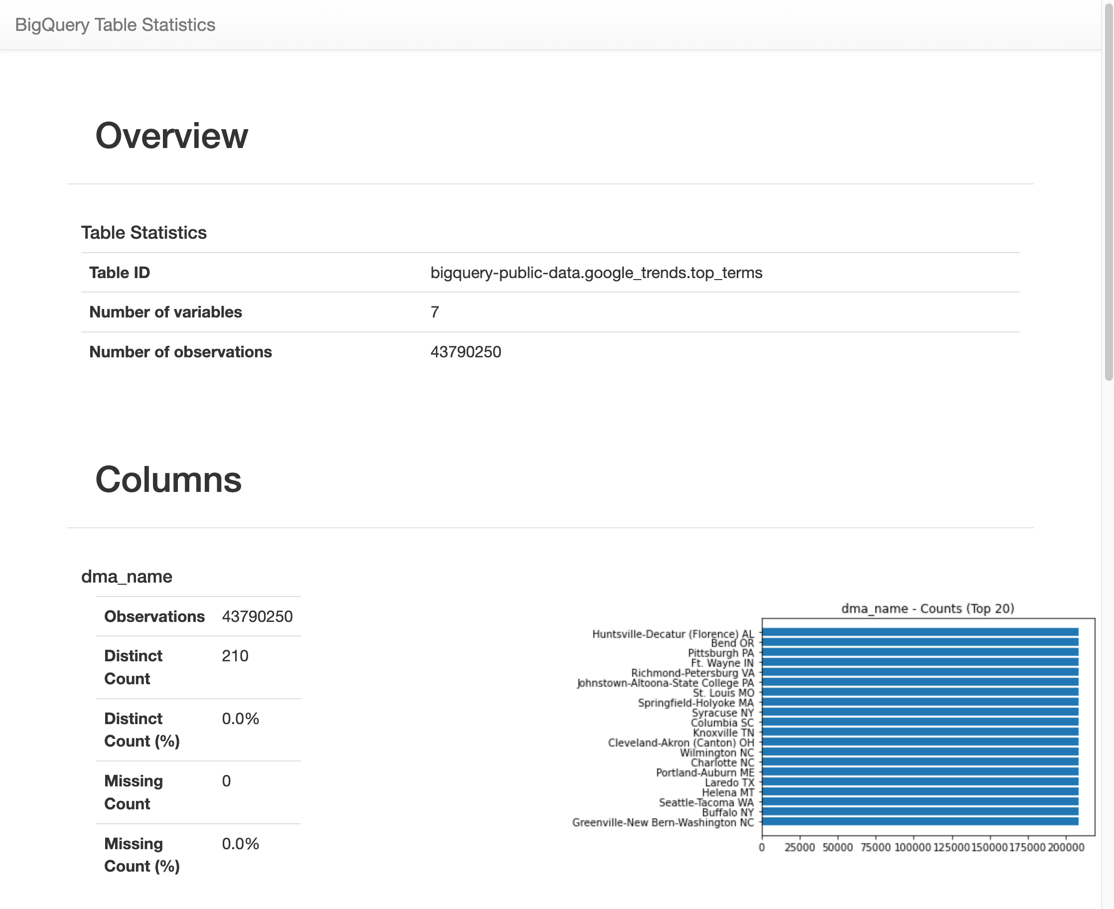

直观呈现 BigQuery 数据

在本部分中，您将使用图表功能直观呈现之前在 Jupyter 笔记本中运行的查询的结果。

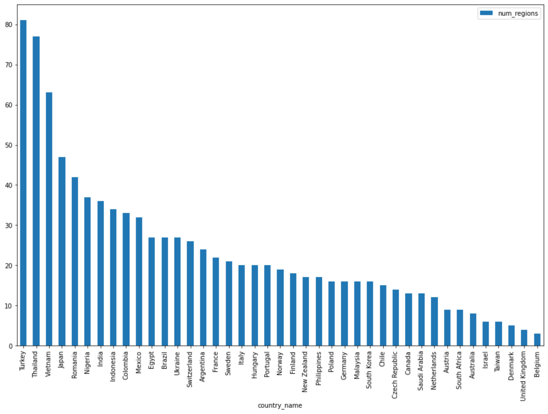
在下一个单元中输入以下代码，以便使用 Pandas DataFrame.plot() 方法创建条形图，用于直观呈现按国家/地区返回区域数的查询结果：
```
regions_by_country.plot(kind="bar", x="country_name", y="num_regions", figsize=(15, 10))
```
点击 运行单元。

图表类似于以下内容：
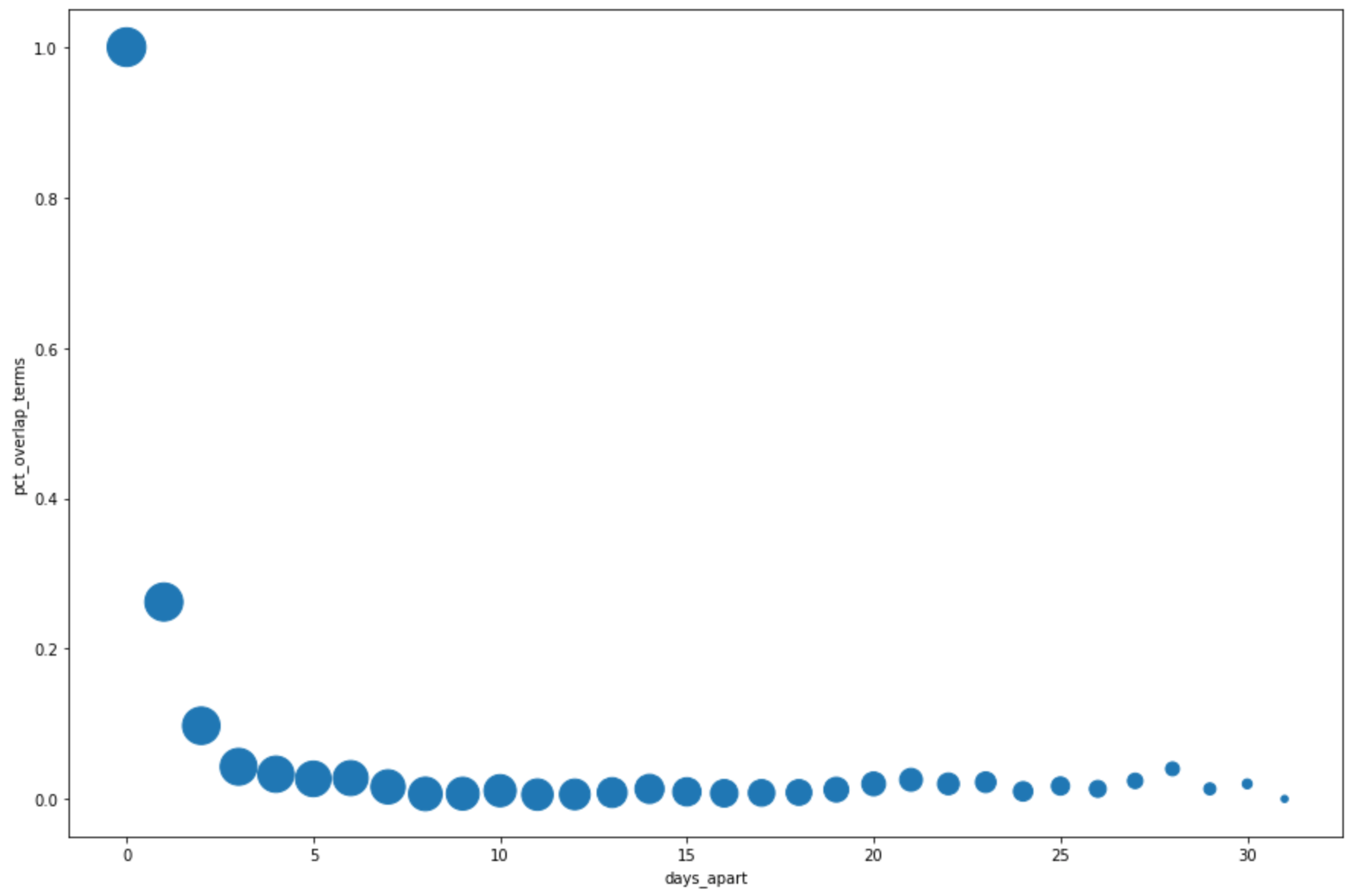
在下一个单元中输入以下代码，以便使用 pandas DataFrame.plot() 方法创建散点图，以直观呈现热门搜索字词在以固定天数为单位的时间段中重叠百分比的查询结果。
```
pct_overlap_terms_by_days_apart.plot(
  kind="scatter",
  x="days_apart",
  y="pct_overlap_terms",
  s=len(pct_overlap_terms_by_days_apart["num_date_pairs"]) * 20,
  figsize=(15, 10)
  )
```
点击 运行单元。

图表类似于以下内容。每个点的大小反映了数据中以较多天数为时间单位的时间段中日期对的数量。例如，以 1 天为时间单位的时间段中的日期对数量多于以以 30 天为时间单位的时间段中的日期对数量，系统会提供更多句对，因为在一个月的时间中每天提供热门搜索字词。

如需详细了解数据可视化，请参阅 Pandas 文档。