Visualize BigQuery GEOGRAPHY polygons with Looker Studio

This tutorial is intended for people who want to visualize GEOGRAPHY data from BigQuery using Looker Studio. To complete this tutorial, you'll need a BigQuery billing project. You don't need to know how to write SQL, and you can use the public dataset.

Goals

In this tutorial, you'll create a report that shows the affordability of rental properties in Washington state. You'll use a Google Map to visualize GEOGRAPHY data coming from a public BigQuery dataset.

In this tutorial, you'll accomplish the following:

• Create a new blank report
• Add a Google Map to the report
• Configure the map
• Style the map
• Interact with the map
• Change the tooltip
• Add more style to the map

Before you begin

If you don't already have a BigQuery billing project set up, you can sign up for free.

Create a new blank report

1. Sign in to Looker Studio.
2. Click Create and then select Report.

3. In the Add data to report panel, choose BigQuery.

   

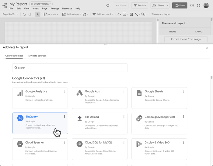
4. In the left navigation, choose CUSTOM QUERY.

5. Select or enter your billing project ID.

6. Under Enter Custom Query, paste the following SQL query:

       select
           ct.state_fips_code,
           ct.county_fips_code,
           c.county_name,
           ct.tract_ce,
           ct.geo_id,
           ct.tract_name,
           ct.lsad_name,
           ct.internal_point_lat,
           ct.internal_point_lon,
           ct.internal_point_geo,
           ct.tract_geom,
           acs.total_pop,
           acs.households,
           acs.male_pop,
           acs.female_pop,
           acs.median_age,
           acs.median_income,
           acs.income_per_capita,
           acs.gini_index,
           acs.owner_occupied_housing_units_median_value,
           acs.median_rent,
           acs.percent_income_spent_on_rent,
       from `bigquery-public-data.geo_census_tracts.census_tracts_washington` ct
       left join `bigquery-public-data.geo_us_boundaries.counties` c
           on (ct.state_fips_code || ct.county_fips_code) = c.geo_id
       left join `bigquery-public-data.census_bureau_acs.censustract_2018_5yr` acs
           on ct.geo_id = acs.geo_id
   

7. Click Add to add this data to the report.

Add a Google Map to the report

1. Delete the table on the report page.
2. Click Add a chart.
3. In the Google Maps section, click Filled map.

Configure the map

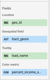
The map won't appear yet. You'll need to add the field that uniquely identifies each location first.

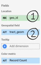
1. In the Location section, click Invalid dimension, and then choose geo_id.
   1. This field uniquely identifies each census tract.
2. In the Geospatial field section, click Add metric, and then choose tract_geom.
   1. This field contains the BigQuery GEOGRAPHY data that defines the polygons that you want to display.

The map should look like this:

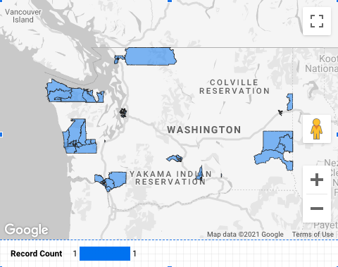
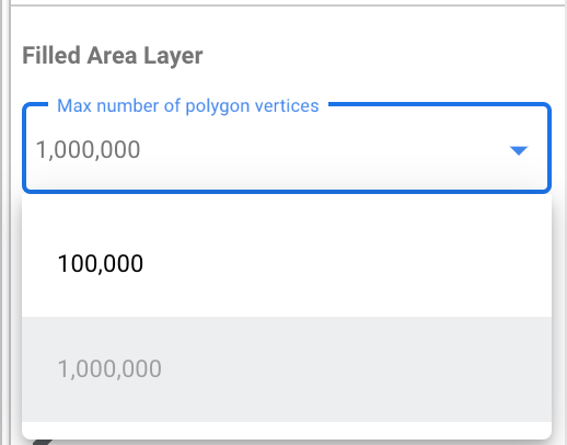
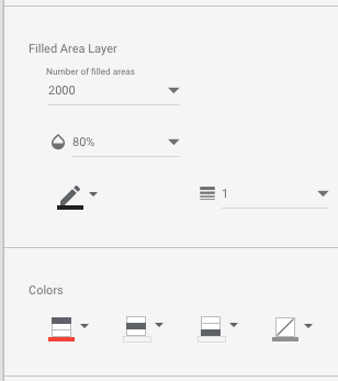
Why is the map missing polygons? A Google Map in Looker Studio plots 100K points (polygon vertices) by default, but the tract_geom column contains 911,364 points. You can increase the number of points (up to a maximum of 1 million) or, to reduce the number of points, you can add a filter to focus on a specific area. In the STYLE tab of the chart properties panel, in the Filled Area Layer section, set the Max number of polygon vertices to 1,000,000.

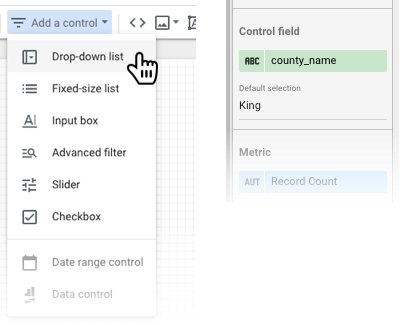
Add a county filter

1. In the toolbar, click Add a control.
2. Select Drop-down list.
3. Set the Control field to county_name, and, for Default selection, enter King.

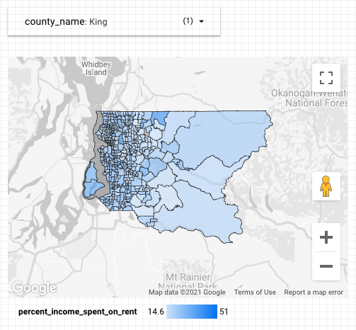
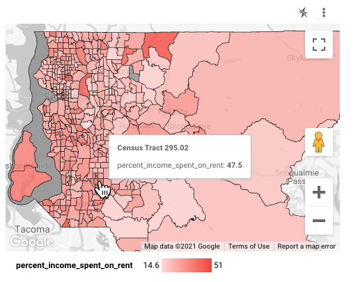
Now you should see all polygons for King County, which contains Seattle:

Style the map

The map's default color metric is Record Count. You can also choose a different metric.

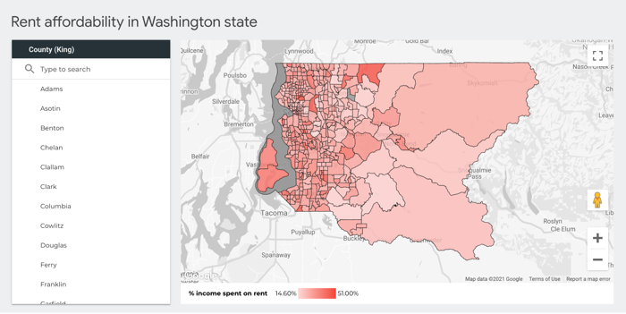
In the Color metric section, choose percent_income_spent_on_rent.

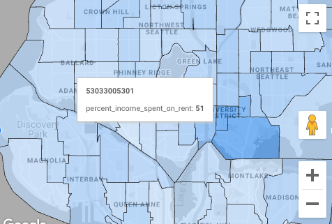
Interact with the map

Depending on the options that you turned on, you can zoom and pan around and notice census tracts where people spend nearly half their income on rent, such as the University District in Seattle:

Change the tooltip

As you mouse over the map, you'll notice that the tooltip shows the geo_id, which isn't particularly meaningful in this context:

You can provide viewers with a more useful tooltip by changing the Tooltip dimension.

1. In the report, click Edit.
2. Select the map.
3. In the Tooltip section of the properties panel, choose lsad_name.
   1. This field contains the human-readable census tract name:

Add more style to the map

You can customize the appearance of the map in the STYLE tab. For example, you could increase the fill opacity to 80% and change the color gradient from blue to red.

Congratulations

You've created a Google Map in Looker Studio that visualizes BigQuery GEOGRAPHY data.

Related resources

• Connect to Google BigQuery
• BigQuery Public Datasets (several datasets with geographic polygon data)
• Google Maps reference
• BigQuery geography functions